Model scope
lmmix fits Gaussian linear mixed models with random
effects, structured residual covariance, or both components in the same
model. The package directly optimizes a profiled ML or REML objective
and does not delegate estimation to another mixed-model package.
This vignette focuses on practical use. The mathematical formulation, covariance parameterizations, likelihood criteria, and inference derivations are presented separately in the vignette Estimation and inference in lmmix.
Prepare the data
The included multicentre data have three treatments,
three measurement occasions, three centers and subjects nested within
center and treatment.
str(multicentre)
#> 'data.frame':    153 obs. of  5 variables:
#>  $ Center : Factor w/ 3 levels "R","S","T": 1 1 1 1 1 1 1 1 1 1 ...
#>  $ Drug   : Factor w/ 3 levels "1","2","3": 1 1 1 1 1 1 1 1 1 1 ...
#>  $ Subject: Factor w/ 8 levels "1","2","3","4",..: 1 1 1 2 2 2 3 3 3 4 ...
#>  $ Time   : Factor w/ 3 levels "1","2","3": 1 2 3 1 2 3 1 2 3 1 ...
#>  $ Y      : num  17 NA NA 12 14 15 12 11 14 13 ...
colSums(is.na(multicentre))
#>  Center    Drug Subject    Time       Y
#>       0       0       0       0      28
The fixed, random and repeated formulas jointly determine the
variables used by the analysis. Missing rows are handled with
na.omit, na.exclude, or na.fail.
The default is na.omit; na.exclude restores
omitted positions in fitted values, residuals, and augmented data.
Fit a combined covariance model
This model contains a random center intercept and an AR(1) residual covariance within subject.
fit <- lmm(
  data = multicentre,
  formula = Y ~ Drug * Time,
  random = ~ 1 | Center,
  repeated = ~ Time | Center:Drug:Subject,
  structure = "ar1",
  method = "REML",
  ddf = "satterthwaite"
)

fit
#> Linear mixed model fit by REML
#> Formula: Y ~ Drug * Time
#> Random (Center): ~1 | Center
#> Repeated: ~Time | Center:Drug:Subject (AR1)
#> Log-likelihood: -245.313
#> Convergence code: 0
The three formulas have distinct roles:
| Argument | Role in the fitted model |
|---|---|
formula |
Defines the response and fixed-effects matrix
X
|
random |
Defines the random-effects matrix Z and
grouping factor for G
|
repeated |
Defines the ordering variable and independent blocks
for R
|
For the residual structures other than id, each
repeated-measures group must have at most one observation per ordering
value.
Inspect convergence before inference
The optimizer code and Hessian diagnostic are part of the fitted object.
fit$convergence[c(
  "code",
  "message",
  "optimizer",
  "iterations",
  "hessian_positive_definite"
)]
#> $code
#> [1] 0
#>
#> $message
#> [1] "relative convergence (4)"
#>
#> $optimizer
#> [1] "nlminb"
#>
#> $iterations
#> [1] 13
#>
#> $hessian_positive_definite
#> [1] TRUE
fit$convergence$attempts
#> # A tibble: 1 × 6
#>   attempt optimizer method convergence objective selected
#>     <int> <chr>     <chr>        <int>     <dbl> <lgl>
#> 1       1 nlminb    NA               0      245. TRUE
A nonzero convergence code or a non-positive-definite likelihood Hessian requires investigation before interpreting standard errors or denominator degrees of freedom. The fitting function emits a warning in either case.
Fixed effects and type III tests
summary() combines coefficient-level inference, type III
tests, covariance parameters and information criteria.
summary(fit)
#> Linear mixed model
#> Estimation: REML
#> Denominator df: satterthwaite
#> Residual covariance: AR1
#>
#> Fixed effects
#> # A tibble: 9 × 8
#>   Term     Estimate `Std Error` Statistic    DF `p value` `Conf Low` `Conf High`
#>   <chr>       <dbl>       <dbl>     <dbl> <dbl>     <dbl>      <dbl>       <dbl>
#> 1 (Interc…   12.1         1.54      7.83   3.06   4.05e-3      7.21       16.9
#> 2 Drug2       4.76        1.12      4.25  49.8    9.28e-5      2.51        7.02
#> 3 Drug3       3.94        1.12      3.52  49.8    9.39e-4      1.69        6.19
#> 4 Time2       0.921       0.294     3.13  67.5    2.55e-3      0.335       1.51
#> 5 Time3       2.39        0.441     5.42  72.1    7.50e-7      1.51        3.27
#> 6 Drug2:T…   -0.143       0.438    -0.326 67.9    7.46e-1     -1.02        0.732
#> 7 Drug3:T…   -0.474       0.448    -1.06  68.0    2.94e-1     -1.37        0.421
#> 8 Drug2:T…    0.823       0.666     1.24  72.7    2.21e-1     -0.505       2.15
#> 9 Drug3:T…    0.334       0.644     0.519 73.1    6.05e-1     -0.949       1.62
#> Type III tests
#> # A tibble: 3 × 5
#>   Term      `Num DF` `Den DF` Statistic `p value`
#>   <chr>        <dbl>    <dbl>     <dbl>     <dbl>
#> 1 Drug             2     46.4     11.4   9.23e- 5
#> 2 Time             2     68.5     59.3   1.16e-15
#> 3 Drug:Time        4     68.4      1.35  2.60e- 1
#> Covariance parameters
#> # A tibble: 3 × 5
#>   Group    Term        Component Estimate `Std Error`
#>   <chr>    <chr>       <chr>        <dbl>       <dbl>
#> 1 Center   (Intercept) var          5.17       5.73
#> 2 Residual ar1         var         10.7        2.14
#> 3 Residual ar1         cor          0.935      0.0169
#> Information criteria
#>    logLik       AIC       BIC  deviance
#> -245.3129  514.6257  548.5655  490.6257
Individual components are also available through standard methods.
fixef(fit)
#> (Intercept)       Drug2       Drug3       Time2       Time3 Drug2:Time2
#>  12.0523813   4.7647059   3.9411765   0.9210921   2.3922321  -0.1427492
#> Drug3:Time2 Drug2:Time3 Drug3:Time3
#>  -0.4735142   0.8233159   0.3342516
vcov(fit)
#>             (Intercept)       Drug2       Drug3       Time2       Time3
#> (Intercept)  2.36770789 -0.62765704 -0.62765704 -0.04061944 -0.07860349
#> Drug2       -0.62765704  1.25531407  0.62765704  0.04072244  0.07880281
#> Drug3       -0.62765704  0.62765704  1.25531407  0.04072244  0.07880281
#> Time2       -0.04061944  0.04072244  0.04072244  0.08637707  0.08342200
#> Time3       -0.07860349  0.07880281  0.07880281  0.08342200  0.19477318
#> Drug2:Time2  0.03995755 -0.08144488 -0.04072244 -0.08637954 -0.08342678
#> Drug3:Time2  0.04056091 -0.04072244 -0.08144488 -0.08639642 -0.08345945
#> Drug2:Time3  0.07663525 -0.15760561 -0.07880281 -0.08341364 -0.19475700
#> Drug3:Time3  0.07849022 -0.07880281 -0.15760561 -0.08345945 -0.19484566
#>             Drug2:Time2 Drug3:Time2 Drug2:Time3 Drug3:Time3
#> (Intercept)  0.03995755  0.04056091  0.07663525  0.07849022
#> Drug2       -0.08144488 -0.04072244 -0.15760561 -0.07880281
#> Drug3       -0.04072244 -0.08144488 -0.07880281 -0.15760561
#> Time2       -0.08637954 -0.08639642 -0.08341364 -0.08345945
#> Time3       -0.08342678 -0.08345945 -0.19475700 -0.19484566
#> Drug2:Time2  0.19210287  0.08639556  0.18498607  0.08345780
#> Drug3:Time2  0.08639556  0.20075228  0.08339410  0.19311444
#> Drug2:Time3  0.18498607  0.08339410  0.44392008  0.19471919
#> Drug3:Time3  0.08345780  0.19311444  0.19471919  0.41428424
anova(fit)
#> Type III tests with satterthwaite degrees of freedom
#> # A tibble: 3 × 5
#>   Term      `Num DF` `Den DF` Statistic `p value`
#>   <chr>        <dbl>    <dbl>     <dbl>     <dbl>
#> 1 Drug             2     46.4     11.4   9.23e- 5
#> 2 Time             2     68.5     59.3   1.16e-15
#> 3 Drug:Time        4     68.4      1.35  2.60e- 1
confint(fit)
#>                  Lower      Upper
#> (Intercept)  7.2059109 16.8988517
#> Drug2        2.5140873  7.0153244
#> Drug3        1.6905579  6.1917950
#> Time2        0.3345435  1.5076408
#> Time3        1.5124810  3.2719833
#> Drug2:Time2 -1.0173805  0.7318821
#> Drug3:Time2 -1.3675896  0.4205612
#> Drug2:Time3 -0.5046493  2.1512811
#> Drug3:Time3 -0.9485017  1.6170050
confint(fit, parm = "theta_")
#>                            Lower      Upper
#> random.var.(Intercept) 0.5898096 45.3849861
#> residual.var           7.2045422 15.8028806
#> residual.cor           0.8923747  0.9612359
anova() performs type III fixed-effect tests for one
model. With multiple models it performs likelihood-ratio comparisons,
automatically refitting REML models with ML when their fixed effects
differ. Satterthwaite, Kenward-Roger, and residual denominator degrees
of freedom are available. Kenward-Roger is restricted to REML fits.
fit_kr <- lmm(
  data = multicentre,
  formula = Y ~ Drug * Time,
  random = ~ 1 | Center,
  repeated = ~ Time | Center:Drug:Subject,
  structure = "ar1",
  ddf = "kenward-roger"
)

fit_reduced <- lmm(
  data = multicentre,
  formula = Y ~ Drug + Time,
  random = ~ 1 | Center,
  repeated = ~ Time | Center:Drug:Subject,
  structure = "ar1"
)
anova(fit_reduced, fit)

# Use a simulated null reference for a covariance comparison.
anova(
  smaller_ml_fit,
  larger_ml_fit,
  test = "parametric.bootstrap",
  nsim = 999,
  seed = 2026
)
Covariance parameters and random effects
VarCorr() returns the estimated covariance components on
their natural scale. ranef() always returns a named list
with one tibble per random term. This stable contract also applies when
the model has only one random term; a marginal model returns an empty
list.
VarCorr(fit)
#> # A tibble: 3 × 5
#>   Group    Term        Component Estimate `Std Error`
#>   <chr>    <chr>       <chr>        <dbl>       <dbl>
#> 1 Center   (Intercept) var          5.17       5.73
#> 2 Residual ar1         var         10.7        2.14
#> 3 Residual ar1         cor          0.935      0.0169
ranef(fit)
#> $Center
#> # A tibble: 3 × 2
#>   Center `(Intercept)`
#>   <chr>          <dbl>
#> 1 R              0.901
#> 2 S              1.55
#> 3 T             -2.45
ranef(fit)[[1L]]
#> # A tibble: 3 × 2
#>   Center `(Intercept)`
#>   <chr>          <dbl>
#> 1 R              0.901
#> 2 S              1.55
#> 3 T             -2.45
For a random-slope model, the random-effect covariance is
unstructured. Its variances and correlations appear as separate rows in
VarCorr().
Estimated marginal means
Marginal means use equal weights over nuisance-factor levels. Numeric
covariates not requested in specs are held at their
observed means. This construction targets population marginal means in
the sense of Searle et al. (1980).
lsmeans(fit, ~Drug)
#> # A tibble: 3 × 8
#>   Drug  Estimate `Std Error`    DF Statistic `p value` `Conf Low` `Conf High`
#>   <fct>    <dbl>       <dbl> <dbl>     <dbl>     <dbl>      <dbl>       <dbl>
#> 1 1         13.2        1.53  2.98      8.60   0.00339       8.27        18.0
#> 2 2         18.1        1.53  3.01     11.8    0.00128      13.3         23.0
#> 3 3         17.1        1.53  3.01     11.1    0.00154      12.2         21.9
lsmeans(fit, ~Time)
#> # A tibble: 3 × 8
#>   Time  Estimate `Std Error`    DF Statistic `p value` `Conf Low` `Conf High`
#>   <fct>    <dbl>       <dbl> <dbl>     <dbl>     <dbl>      <dbl>       <dbl>
#> 1 1         15.0        1.40  2.08      10.7   0.00753       9.16        20.8
#> 2 2         15.7        1.40  2.09      11.2   0.00670       9.90        21.4
#> 3 3         17.7        1.40  2.12      12.6   0.00495      12.0         23.5
Pairwise contrast matrices are generated automatically. The
adjust argument is passed to
stats::p.adjust(). When p-values are adjusted,
conf_adjust = "auto" reports simultaneous Bonferroni
confidence intervals. Use conf_adjust = "none" for
pointwise intervals.
lsmeans(fit, pairwise ~ Drug, adjust = "holm")
#> Estimated marginal means
#> # A tibble: 3 × 8
#>   Drug  Estimate `Std Error`    DF Statistic `p value` `Conf Low` `Conf High`
#>   <fct>    <dbl>       <dbl> <dbl>     <dbl>     <dbl>      <dbl>       <dbl>
#> 1 1         13.2        1.53  2.98      8.60   0.00339       8.27        18.0
#> 2 2         18.1        1.53  3.01     11.8    0.00128      13.3         23.0
#> 3 3         17.1        1.53  3.01     11.1    0.00154      12.2         21.9
#> Pairwise contrasts
#> P-value adjustment: holm; confidence intervals: bonferroni
#> # A tibble: 3 × 8
#>   Contrast Estimate `Std Error`    DF Statistic `p value` `Conf Low` `Conf High`
#>   <chr>       <dbl>       <dbl> <dbl>     <dbl>     <dbl>      <dbl>       <dbl>
#> 1 1 - 2       -4.99        1.10  46.1    -4.54   0.000120      -7.72       -2.26
#> 2 1 - 3       -3.89        1.10  46.1    -3.54   0.00183       -6.62       -1.16
#> 3 2 - 3        1.10        1.10  46.9     0.993  0.326         -1.64        3.84
Reference values for numeric covariates can be overridden with
at:
When emmeans is installed, lmmix supplies
the required fixed-effects basis and model-specific denominator degrees
of freedom.
emmeans::emmeans(fit, ~Drug)
#> NOTE: Results may be misleading due to involvement in interactions
#>  Drug emmean   SE   df lower.CL upper.CL
#>  1      13.2 1.53 2.98     8.27     18.0
#>  2      18.1 1.53 3.01    13.28     23.0
#>  3      17.1 1.53 3.01    12.18     21.9
#>
#> Results are averaged over the levels of: Time
#> Confidence level used: 0.95
Predictions, residuals and tidy output
Conditional fitted values include empirical random effects. Marginal fitted values use fixed effects only.
head(fitted(fit, type = "conditional"))
#>        1        4        5        6        7        8
#> 12.95368 12.95368 13.87477 15.34591 12.95368 13.87477
head(fitted(fit, type = "marginal"))
#>        1        4        5        6        7        8
#> 12.05238 12.05238 12.97347 14.44461 12.05238 12.97347
head(residuals(fit, type = "pearson"))
#>           1           4           5           6           7           8
#>  1.23872457 -0.29195520  0.03833728 -0.10589561 -0.29195520 -0.88007058
For predict(fit, newdata), known grouping levels receive
their fitted random effect. New groups cause an error unless
allow.new.levels = TRUE is supplied; when allowed, their
random contribution is zero. Use re.form = NA or
re.form = ~ 0 for fixed-effects-only predictions. A fitted
random-effects formula, or a list of fitted formulas, selects a subset
of random terms.
Standard errors and intervals are available directly. Confidence
intervals describe the expected response. Prediction intervals
additionally include the fitted residual variance. Both condition on
empirical random effects selected through re.form; BLUP
estimation uncertainty is not added.
Simulation, updating, weights, and offsets
simulate() draws marginal Gaussian response vectors from
the fitted mean and covariance. Supplying a seed makes the result
reproducible without changing the caller’s random-number state.
update() refits a modified formula or model argument.
Known relative precision weights rescale the residual covariance on
both sides by diag(1 / sqrt(weights)). Formula offsets,
explicit offsets, and custom fixed-effect contrasts are also
supported.
Diagnostic plots
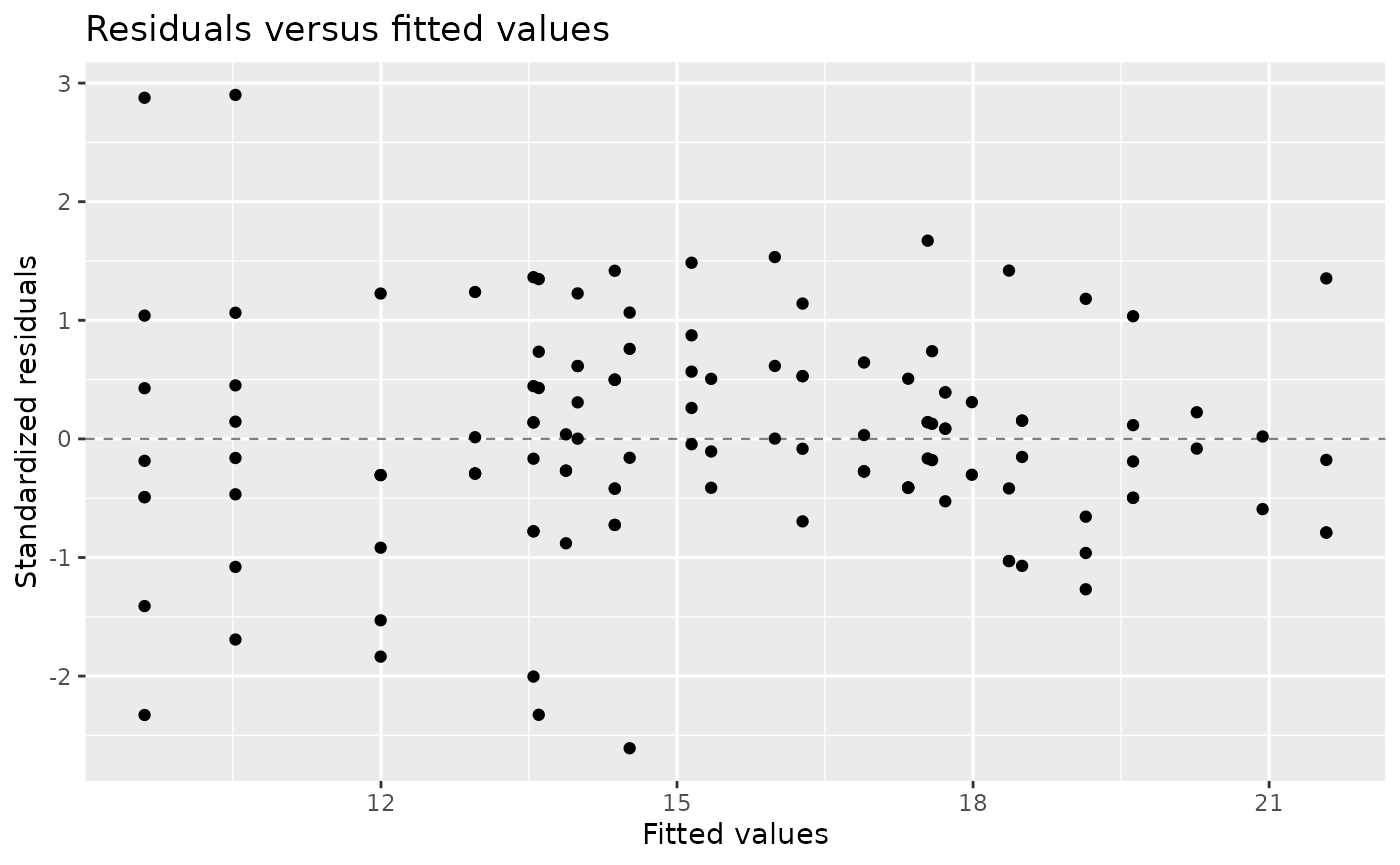
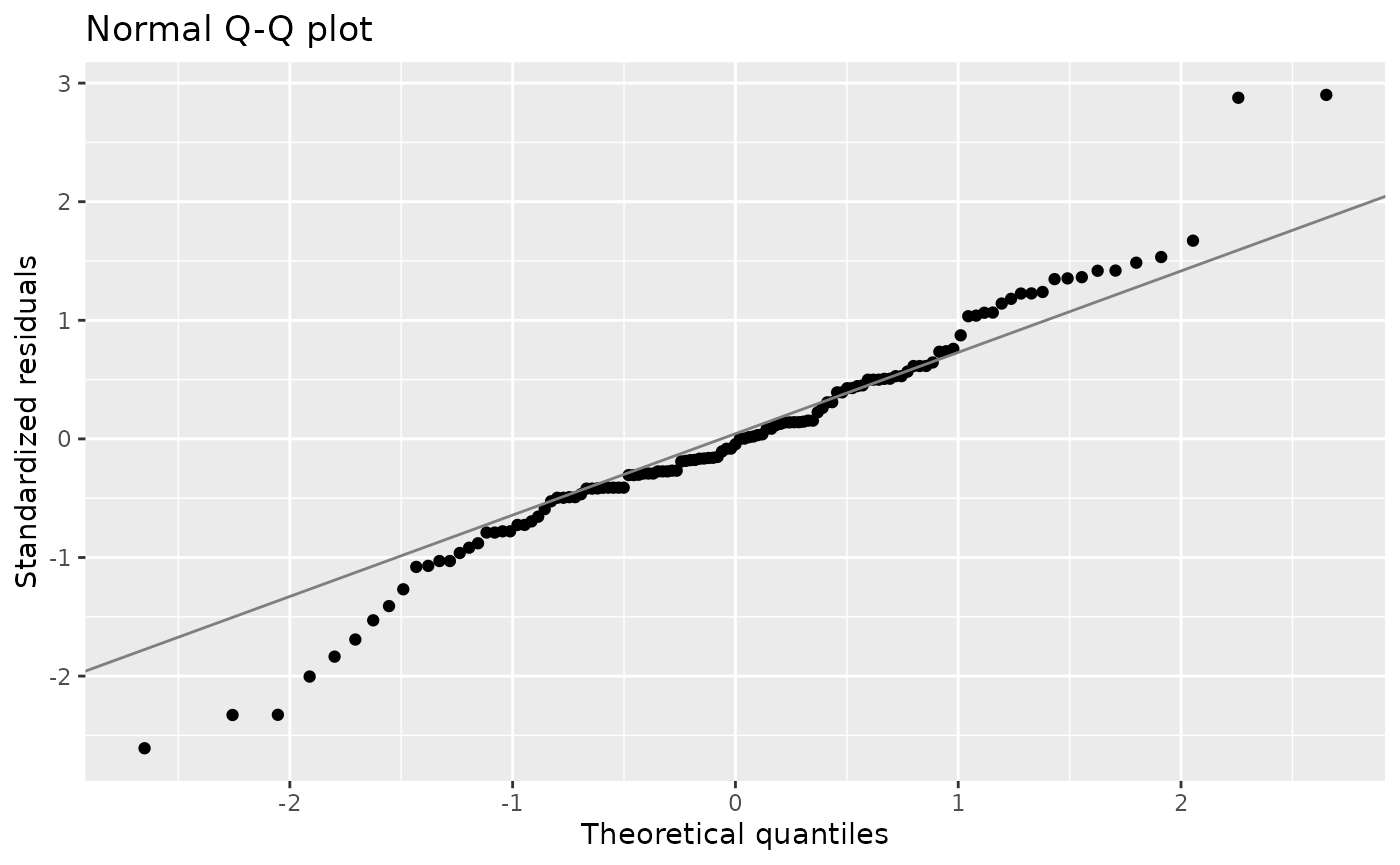
The S3 method plot.lmm() returns a ggplot2
object. Three diagnostics are available through which:
standardized residuals against fitted values, a normal Q-Q plot, and
observed against fitted values.
Because the returned object is a ggplot, layers and
themes can be added in the usual way.
plot(fit, which = "fitted") +
  ggplot2::theme_minimal()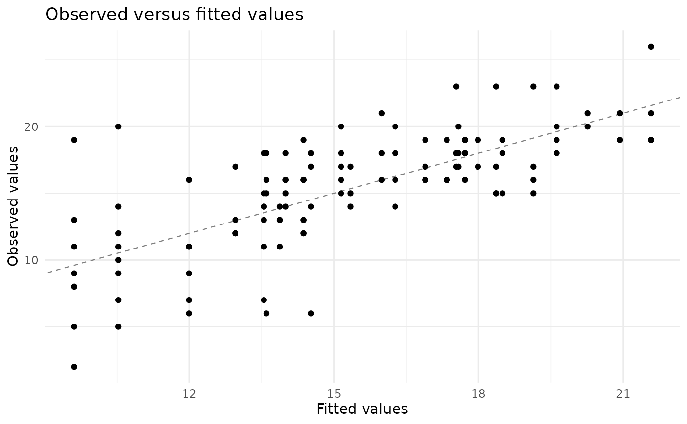
For correlated residual structures, the plotted Pearson residuals are scaled by their marginal residual standard deviations. They are not decorrelated innovations, so residual dependence should also be assessed within the repeated-measures groups.
The generics methods return tibbles.
Printed tables use readable headings without dots, such as
Std Error, p value, Conf Low, and
Conf High. The underlying tibbles retain the standard
broom column names required for programmatic use. Input
column names are preserved by augment() and
ranef().
generics::tidy(fit)
#> # A tibble: 9 × 7
#>   Effect Term        Estimate `Std Error` Statistic    DF   `p value`
#>   <chr>  <chr>          <dbl>       <dbl>     <dbl> <dbl>       <dbl>
#> 1 fixed  (Intercept)   12.1         1.54      7.83   3.06 0.00405
#> 2 fixed  Drug2          4.76        1.12      4.25  49.8  0.0000928
#> 3 fixed  Drug3          3.94        1.12      3.52  49.8  0.000939
#> 4 fixed  Time2          0.921       0.294     3.13  67.5  0.00255
#> 5 fixed  Time3          2.39        0.441     5.42  72.1  0.000000750
#> 6 fixed  Drug2:Time2   -0.143       0.438    -0.326 67.9  0.746
#> 7 fixed  Drug3:Time2   -0.474       0.448    -1.06  68.0  0.294
#> 8 fixed  Drug2:Time3    0.823       0.666     1.24  72.7  0.221
#> 9 fixed  Drug3:Time3    0.334       0.644     0.519 73.1  0.605
generics::glance(fit)
#> # A tibble: 1 × 8
#>   `Log Lik`   AIC   BIC Deviance    DF `N Obs` Convergence Method
#>       <dbl> <dbl> <dbl>    <dbl> <int>   <int>       <int> <chr>
#> 1     -245.  515.  549.     491.    12     125           0 REML
head(generics::augment(fit))
#> # A tibble: 6 × 8
#>   Center Drug  Subject Time      Y Fitted Residual `Std Residual`
#>   <fct>  <fct> <fct>   <fct> <dbl>  <dbl>    <dbl>          <dbl>
#> 1 R      1     1       1        17   13.0    4.05          1.24
#> 2 R      1     2       1        12   13.0   -0.954        -0.292
#> 3 R      1     2       2        14   13.9    0.125         0.0383
#> 4 R      1     2       3        15   15.3   -0.346        -0.106
#> 5 R      1     3       1        12   13.0   -0.954        -0.292
#> 6 R      1     3       2        11   13.9   -2.87         -0.880
Alternative model specifications
The same interface covers marginal, random-effects and combined models.
# Marginal model with unstructured repeated-measures covariance
fit_marginal <- lmm(
  data,
  response ~ treatment * time,
  repeated = ~ time | subject,
  structure = "un"
)

# Random intercept and slope with independent residuals
fit_random <- lmm(
  data,
  response ~ treatment + time,
  random = ~ 1 + time | subject,
  structure = "id"
)

# Independent crossed random intercepts
fit_crossed <- lmm(
  data,
  response ~ treatment + time,
  random = list(
    center = ~ 1 | center,
    subject = ~ 1 | subject
  )
)

# Combined random intercept and Toeplitz residual covariance
fit_combined <- lmm(
  data,
  response ~ treatment * time,
  random = ~ 1 | center,
  repeated = ~ time | center:subject,
  structure = "toep"
)

# Four-band Toeplitz covariance, including the main diagonal
fit_banded <- lmm(
  data,
  response ~ treatment * time,
  random = ~ 1 | center,
  repeated = ~ time | center:subject,
  structure = "toep(4)"
)
Practical limits
Version 0.4.0 identifies independent connected
components induced by the random and repeated grouping structures. The
likelihood is evaluated by factoring one covariance matrix per component
and aggregating their GLS contributions. This substantially reduces work
for many subject-level or nested designs.
The fitted object still stores the complete dense marginal
covariance, and some inference calculations remain dense. Crossed
effects can connect all observations into one component. Consequently,
lmmix is not yet a large-scale sparse mixed-model engine
and does not promise a fixed observation limit. The practical cost
depends on the size of the largest connected component, the number of
covariance parameters, and the requested inference. Generalized
responses remain outside the Gaussian model scope.