DonutMap creates donut charts positioned on a map from tidy data. The package has three main workflows:
-
donut_polygons()creates ansfpolygon layer. -
donut_map()creates a staticggplot2map. -
donut_leaflet()creates an interactiveleafletmap with clickable donut segments and optional links or curved trajectories.
The examples below use a Natural Earth boundary loaded with
rnaturalearth (Natural Earth, n.d., https://www.naturalearthdata.com/). The point-level
category values and origin-destination trajectories are simulated for
demonstration.
library(DonutMap)
library(ggplot2)
library(sf)
#> Linking to GEOS 3.12.1, GDAL 3.8.4, PROJ 9.4.0; sf_use_s2() is TRUE

set.seed(20260522)
Example data
The input data are tidy: each row gives a value for one category at
one location. Locations can be supplied either as longitude and latitude
columns or as an sf object.
sites <- data.frame(
  site = c("Site A", "Site B", "Site C", "Site D", "Site E"),
  lon = c(-73.57, -71.21, -72.75, -68.52, -66.82),
  lat = c(45.50, 46.81, 45.40, 48.45, 50.22)
)

categories <- c("Walking", "Transit", "Car")

demo <- merge(
  sites,
  data.frame(category = categories),
  by = NULL
)

demo$value <- c(
  32, 48, 120,
  55, 80, 95,
  28, 70, 110,
  20, 44, 76,
  18, 30, 58
)

demo$category <- factor(demo$category, levels = categories)

flows <- data.frame(
  from = c(
    "Site A", "Site A", "Site B", "Site B",
    "Site C", "Site C", "Site D", "Site E"
  ),
  to = c(
    "Site B", "Site C", "Site D", "Site A",
    "Site E", "Site B", "Site E", "Site C"
  ),
  trips = c(180, 90, 120, 75, 70, 55, 60, 45),
  flow_category = c(
    "Transit", "Car", "Walking", "Transit",
    "Car", "Walking", "Walking", "Transit"
  )
)

category_colours <- c(
  Walking = "#1b9e77",
  Transit = "#7570b3",
  Car = "#d95f02"
)
For a background map, this vignette crops the Natural Earth Canada boundary to eastern Canada. The donut values and flow values remain simulated.
canada <- rnaturalearth::ne_countries(
  country = "Canada",
  returnclass = "sf"
)

eastern_canada <- sf::st_crop(
  canada,
  sf::st_bbox(
    c(xmin = -81, ymin = 44, xmax = -62, ymax = 53.5),
    crs = sf::st_crs(4326)
  )
)
#> Warning: attribute variables are assumed to be spatially constant throughout
#> all geometries
Static map
donut_map() returns a normal ggplot object,
so additional ggplot2 layers, scales, labels, and themes
can be added afterwards. The flows argument adds links
between donut locations. flow_group colours those links by
a column in the flow table, which is useful for showing the
municipality, mode, or class of each connection. Use
flow_curvature = 0 for straight links, and larger positive
or negative values for curved trajectories.
donut_map(
  demo,
  site,
  category,
  value,
  lon = lon,
  lat = lat,
  map = eastern_canada,
  crs = 3347,
  radius_range = c(25000, 70000),
  colours = category_colours,
  flows = flows,
  from = from,
  to = to,
  flow_value = trips,
  flow_group = flow_category,
  flow_colours = category_colours,
  flow_linewidth_range = c(0.3, 2.2),
  flow_curvature = 0.22,
  flow_arrow = TRUE
) +
  labs(
    title = "Simulated mobility composition by site",
    fill = "Mode",
    linewidth = "Trips"
  ) +
  theme(legend.position = "right")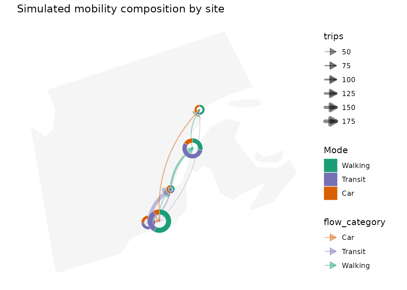
Interactive map
donut_leaflet() returns a leaflet
htmlwidget. Donut segments and trajectory lines, including arrowheads,
can be clicked to open popups, and hover labels are enabled by default.
When flow_group is supplied, both the trajectory lines and
their arrowheads are coloured by group. By default, interactive donuts
are constructed in EPSG:3857, the display projection used by Leaflet,
which keeps the sector boundaries visually regular on screen. Leaflet
simplification is also disabled for donut polygons so the sector borders
are not simplified after the widget is rendered.
donut_leaflet(
  demo,
  site,
  category,
  value,
  lon = lon,
  lat = lat,
  map = eastern_canada,
  radius_range = c(25000, 70000),
  n = 160,
  colours = category_colours,
  flows = flows,
  from = from,
  to = to,
  flow_value = trips,
  flow_group = flow_category,
  flow_colours = category_colours,
  flow_weight_range = c(1, 7),
  flow_curvature = 0.22,
  flow_arrow = TRUE,
  flow_arrow_size = 45000,
  flow_opacity = 0.75
)
Trajectory geometries
flow_lines() returns the trajectory layer directly as an
sf object. This is useful when you want to build a custom
map layer or inspect the geometry before plotting.
trajectories <- flow_lines(
  flows,
  demo,
  from,
  to,
  trips,
  site,
  group = flow_category,
  lon = lon,
  lat = lat,
  crs = 3347,
  flow_curvature = 0.22,
  flow_n = 40
)

trajectories
#> Simple feature collection with 8 features and 4 fields
#> Geometry type: LINESTRING
#> Dimension:     XY
#> Bounding box:  xmin: 7631610 ymin: 1244380 xmax: 7936146 ymax: 1910206
#> Projected CRS: NAD83 / Statistics Canada Lambert
#> # A tibble: 8 × 5
#>   from   to     value group                                             geometry
#>   <chr>  <chr>  <dbl> <chr>                                     <LINESTRING [m]>
#> 1 Site A Site B   180 Transit (7631610 1244380, 7632825 1250853, 7634155 125725…
#> 2 Site A Site C    90 Car     (7631610 1244380, 7633203 1245308, 7634801 124619…
#> 3 Site B Site D   120 Walking (7763098 1440475, 7763754 1448083, 7764551 145561…
#> 4 Site B Site A    75 Transit (7763098 1440475, 7761882 1434001, 7760553 142760…
#> 5 Site C Site E    70 Car     (7697210 1252459, 7696045 1271925, 7695261 129125…
#> 6 Site C Site B    55 Walking (7697210 1252459, 7696833 1258005, 7696564 126351…
#> 7 Site D Site E    60 Walking (7892189 1681853, 7890745 1688166, 7889433 169445…
#> 8 Site E Site C    45 Transit (7933770 1910206, 7934935 1890740, 7935719 187141…
Using the geometry layer directly
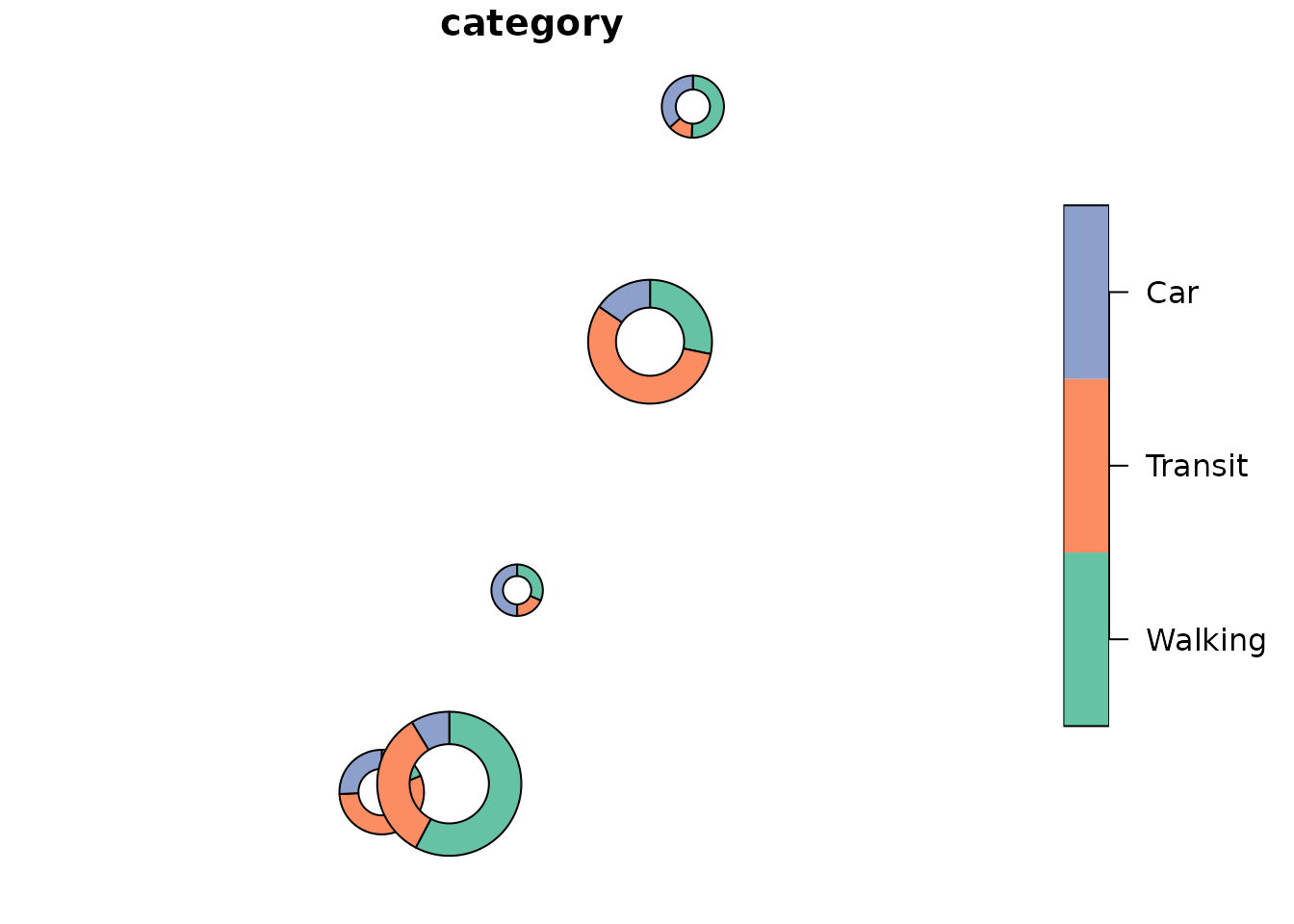
For more specialized workflows, donut_polygons() returns
the donut segments as valid sf polygons.
donuts <- donut_polygons(
  demo,
  site,
  category,
  value,
  lon = lon,
  lat = lat,
  crs = 3347,
  radius_range = c(25000, 70000)
)

donuts
#> Simple feature collection with 15 features and 8 fields
#> Geometry type: POLYGON
#> Dimension:     XY
#> Bounding box:  xmin: 7590543 ymin: 1182476 xmax: 7963944 ymax: 1940386
#> Projected CRS: NAD83 / Statistics Canada Lambert
#> # A tibble: 15 × 9
#>    id     category value total proportion radius start_angle end_angle
#>    <chr>  <fct>    <dbl> <dbl>      <dbl>  <dbl>       <dbl>     <dbl>
#>  1 Site A Walking     32   171     0.187  41076.       1.57      0.395
#>  2 Site A Transit     95   171     0.556  41076.       0.395    -3.10
#>  3 Site A Car         44   171     0.257  41076.      -3.10     -4.71
#>  4 Site B Walking     48   152     0.316  25000        1.57     -0.413
#>  5 Site B Transit     28   152     0.184  25000       -0.413    -1.57
#>  6 Site B Car         76   152     0.5    25000       -1.57     -4.71
#>  7 Site C Walking    120   208     0.577  70000        1.57     -2.05
#>  8 Site C Transit     70   208     0.337  70000       -2.05     -4.17
#>  9 Site C Car         18   208     0.0865 70000       -4.17     -4.71
#> 10 Site D Walking     55   195     0.282  60155.       1.57     -0.201
#> 11 Site D Transit    110   195     0.564  60155.      -0.201    -3.75
#> 12 Site D Car         30   195     0.154  60155.      -3.75     -4.71
#> 13 Site E Walking     80   158     0.506  30180.       1.57     -1.61
#> 14 Site E Transit     20   158     0.127  30180.      -1.61     -2.41
#> 15 Site E Car         58   158     0.367  30180.      -2.41     -4.71
#> # ℹ 1 more variable: geometry <POLYGON [m]>
You can use that object with any package that accepts sf
polygons.
plot(donuts["category"])