Generative validation of SSF / iSSF models
Source:vignettes/generative-validation-ssf.Rmd
generative-validation-ssf.RmdMotivation
Step-selection functions (SSFs) and integrated step-selection analyses (iSSAs) are usually fitted to local, one-step movement decisions. A model can therefore look satisfactory at the scale at which it was fitted while still generating unrealistic trajectories when it is iterated forward. Generative validation asks a direct question: if we simulate full trajectories from the fitted model, do the simulated tracks reproduce important trajectory-level patterns in the observed track?
Nicosia (2026) proposes a multi-criteria framework with four complementary pillars:
- Emergent space use, comparing observed and simulated utilization distributions.
- Diffusion behavior, comparing mean squared displacement (MSD) curves.
- Path structure, comparing path straightness or sinuosity.
- Barrier interactions, comparing intersections with a known linear barrier.
gmov implements these diagnostics for observed and
simulated tracks. It is designed to sit after a modelling workflow such
as amt: users fit an SSF or iSSF, simulate replicate
tracks, and then pass those tracks to gmov.
Red deer empirical example
The empirical application in Nicosia (2026) uses the red deer
trajectory and forest raster distributed with amt (Signer,
Fieberg, and Avgar, 2019). The article fits a standard iSSA to a
GPS-tracked red deer from northern Germany, using a 6-hour sampling
interval, a binary forest covariate, and a 1:25 used-to-available step
design. The fitted model includes forest selection and movement-kernel
terms:
case_ ~ forest + sl_ + log_sl + cos_ta + strata(step_id_)Because the empirical example does not specify a known barrier geometry, the article evaluates the first three pillars: emergent space use, MSD, and sinuosity.
This vignette ships a compact, precomputed version of that red deer
validation example so that the vignette renders with visible results on
installation and on GitHub. The object contains the observed red deer
track, 99 simulated tracks from the empirical iSSA workflow used in the
article, and the scorecard reported by that workflow. The full
amt fitting code is shown later for context.
Load the validation ensemble
data("red_deer_gmov", package = "gmov")

observed_track <- red_deer_gmov$observed_track
simulated_tracks <- red_deer_gmov$simulated_tracks

data.frame(
  observed_locations = nrow(observed_track),
  observed_steps = nrow(observed_track) - 1,
  simulated_tracks = length(simulated_tracks),
  simulated_locations_min = min(vapply(simulated_tracks, nrow, integer(1))),
  simulated_locations_max = max(vapply(simulated_tracks, nrow, integer(1)))
)
#>   observed_locations observed_steps simulated_tracks simulated_locations_min
#> 1                823            822               99                     823
#>   simulated_locations_max
#> 1                     823
The table below is the scorecard from the empirical workflow in Nicosia (2026). It is included as provenance for the precomputed simulation ensemble.
red_deer_gmov$article_scorecard
#>        Pillar      Metric     Observed P_Value       Result
#> 1 1. Topology Wasserstein 5.323038e+03    0.68 NOT REJECTED
#> 2 2. Dynamics   MSD (ISE) 3.229350e+10    0.04     REJECTED
#> 3 3. Behavior   Sinuosity 8.052233e-03    0.17 NOT REJECTED
The article reports a pattern of partial generative realism: the fitted iSSA reproduces broad space-use and path straightness, but shows a detectable mismatch in displacement dynamics.
Observed and simulated trajectories
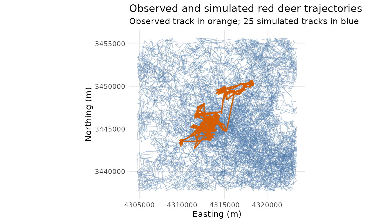
The observed trajectory is shown in orange. A subset of the 99 simulated trajectories is shown in blue to keep the plot readable.
plot_sims <- simulated_tracks[seq_len(25)]
plot_sims_df <- do.call(
  rbind,
  Map(
    function(track, id) {
      data.frame(sim_id = id, x_ = track$x_, y_ = track$y_)
    },
    plot_sims,
    seq_along(plot_sims)
  )
)

ggplot2::ggplot() +
  ggplot2::geom_path(
    data = plot_sims_df,
    ggplot2::aes(x = x_, y = y_, group = sim_id),
    color = col_sim,
    alpha = 0.45,
    linewidth = 0.25
  ) +
  ggplot2::geom_path(
    data = observed_track,
    ggplot2::aes(x = x_, y = y_),
    color = col_obs,
    linewidth = 0.8
  ) +
  ggplot2::coord_equal() +
  ggplot2::theme_minimal() +
  ggplot2::theme(
    panel.grid.minor = ggplot2::element_blank(),
    panel.grid.major = ggplot2::element_line(color = "grey90", linewidth = 0.3)
  ) +
  ggplot2::labs(
    x = "Easting (m)",
    y = "Northing (m)",
    title = "Observed and simulated red deer trajectories",
    subtitle = "Observed track in orange; 25 simulated tracks in blue"
  )
Run the gmov diagnostics
The call below validates the same supplied simulation ensemble with
the current gmov diagnostics. The UD diagnostic uses an
empirical grid approximation to the utilization distribution. The MSD
diagnostic uses lagged MSD curves. These implementation details are
documented in the package help pages, and numerical values can differ
from the prototype diagnostics used in the article.
deer_validation <- validate_ssf_generative(
  observed = observed_track,
  simulated = simulated_tracks,
  metrics = c("ud", "msd", "sinuosity"),
  ud_args = list(grid_size = 20),
  msd_args = list(max_lag = 80)
)

deer_validation
#> gmov generative validation
#> Observed locations: 823
#> Simulated tracks: 99
#> Validation pillars: Emergent space use, Diffusion behavior, Path structure
#>
#> # A tibble: 3 × 7
#>   pillar             metric    diagnostic                      observed
#>   <chr>              <chr>     <chr>                              <dbl>
#> 1 Emergent space use ud        mean observed-simulated grid W1 5.29e+ 3
#> 2 Diffusion behavior msd       MSD integrated squared error    4.12e+15
#> 3 Path structure     sinuosity absolute straightness deviation 8.05e- 3
#>   discrepancy p_value alternative
#>         <dbl>   <dbl> <chr>
#> 1    5.29e+ 3    0.96 greater
#> 2    4.12e+15    0.06 greater
#> 3    1.51e- 2    0.17 greater
The printed object gives a compact diagnostic scorecard with one row per validation pillar. The same information is also available as a tidy tibble for downstream work.
summary(deer_validation)
#> # A tibble: 3 × 6
#>   metric    statistic_name      observed_statistic discrepancy_statistic p_value
#>   <chr>     <chr>                            <dbl>                 <dbl>   <dbl>
#> 1 ud        mean observed-simu…           5.29e+ 3              5.29e+ 3    0.96
#> 2 msd       MSD integrated squ…           4.12e+15              4.12e+15    0.06
#> 3 sinuosity absolute straightn…           8.05e- 3              1.51e- 2    0.17
#> # ℹ 1 more variable: alternative <chr>
Visual diagnostics
The default gmov plots are intentionally simple package
diagnostics. They are not exact reproductions of the custom figures
prepared for the article. Their purpose is to give a stable visual
summary for any gmov_generative object; article-specific
figure layouts can still be built from the returned tidy objects when
needed. The package plots use the same basic visual coding as the
article workflow: blue for simulated quantities and orange for the
observed track or observed statistic.
The UD diagnostic compares the observed grid utilization distribution to the simulated grid utilization distributions using the 1-Wasserstein distance between empirical grid masses.
plot(deer_validation, metric = "ud")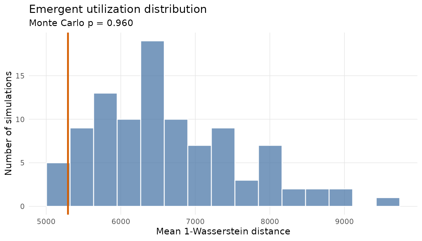
The MSD diagnostic compares the observed lagged displacement curve to the simulation envelope. This targets temporal organization of movement, not only the final spatial footprint.
plot(deer_validation, metric = "msd")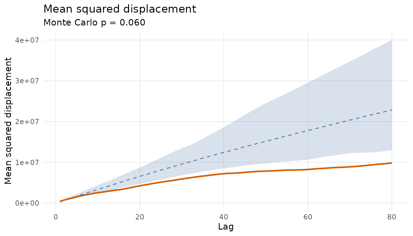
The sinuosity diagnostic compares the observed straightness index with the distribution of straightness indices from simulated trajectories.
plot(deer_validation, metric = "sinuosity")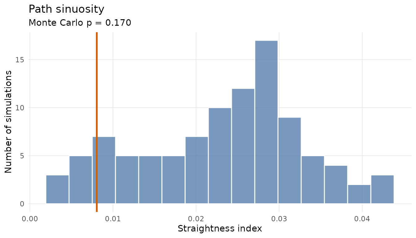
Article-style dashboard
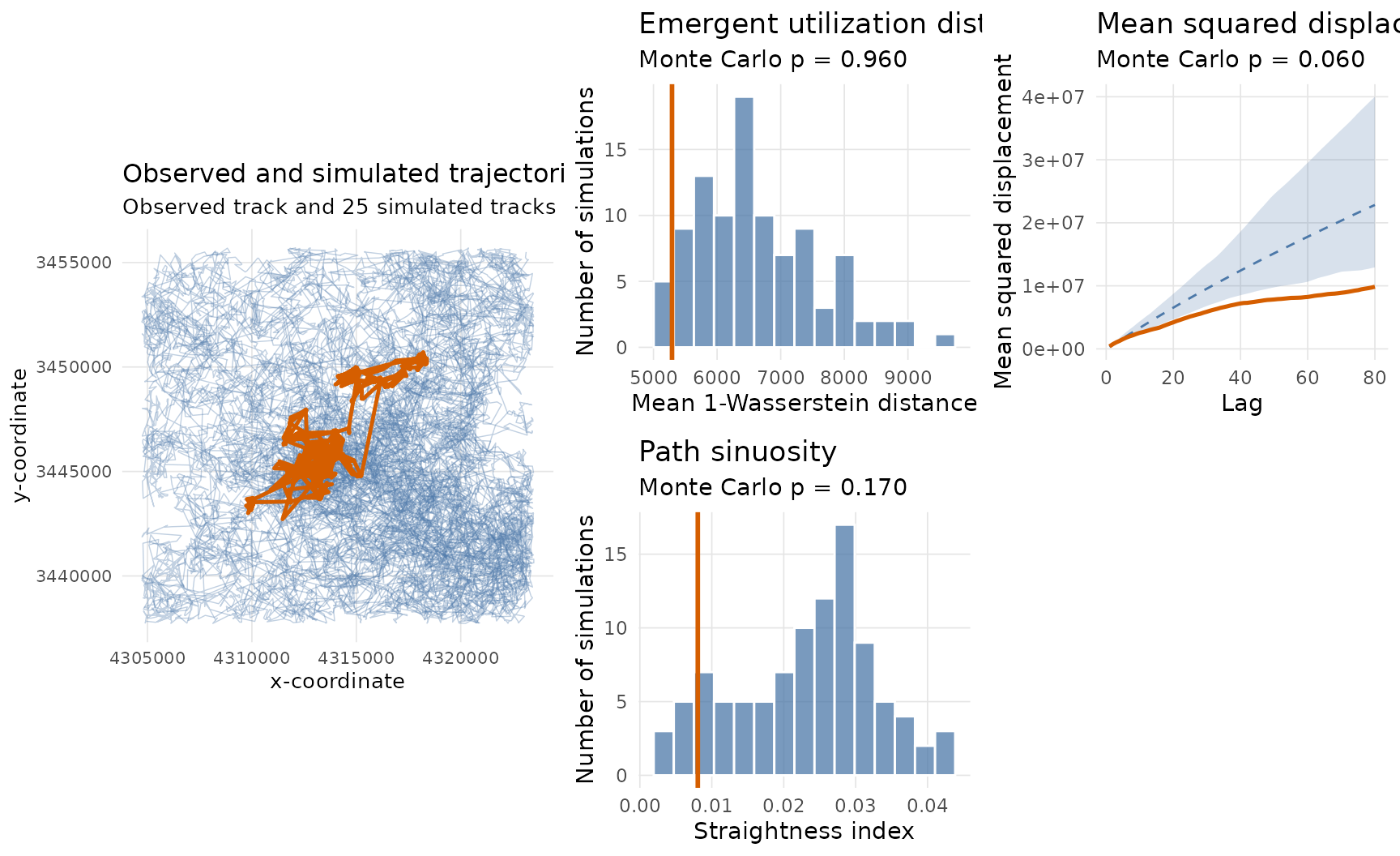
For presentations or reports, the same diagnostics can be displayed
as a compact multi-panel dashboard. This figure keeps the generic
gmov diagnostics but arranges them in a layout closer to
the article workflow: trajectory panel on the left, diagnostic panels on
the right.
plot_gmov_dashboard(
  deer_validation,
  observed = observed_track,
  simulated = simulated_tracks,
  n_simulations = 25
)
Reproducing the model-fitting workflow with amt
The precomputed ensemble above was produced from the red deer and
forest objects distributed with amt. The modelling workflow
is summarized here rather than evaluated during vignette building,
because it depends on a working amt installation and can
take longer than a typical package vignette build.
The empirical workflow used the following steps:
- Load the red deer relocation data and the forest raster distributed
with
amt. - Resample the trajectory to a 6-hour interval with a 30-minute tolerance.
- Convert the resampled trajectory to steps.
- Generate 25 available steps for each observed step.
- Extract the binary forest covariate for used and available steps.
- Add movement-kernel terms for step length, log step length, and cosine of turning angle.
- Fit the iSSA with the conditional logistic regression formula shown above.
- Simulate replicate trajectories from the fitted model.
- Pass the observed trajectory and simulated trajectories to
validate_ssf_generative().
Once the simulation output is a list of track-like objects, the
validation step is the same as in this vignette: call
validate_ssf_generative() with the observed track,
simulated tracks, and selected metrics, then inspect
summary() and plot() outputs.
Interpretation
The red deer example illustrates why generative validation is useful even when a fitted iSSA is plausible at the one-step scale. The model can generate trajectories that occupy broadly similar regions of space while still failing to reproduce the temporal structure of displacement. In the article workflow, this appears as a mismatch in the MSD pillar, while the broad space-use and sinuosity pillars are not rejected.
In practice, the diagnostics should be read together. A single p-value is not a complete model assessment. Instead, the pattern across pillars helps identify which aspect of generative realism is plausible and which aspect may require a better movement kernel, additional behavioural states, temporal structure, or landscape constraints.
References
Avgar, T., Potts, J. R., Lewis, M. A., and Boyce, M. S. (2016). Integrated step selection analysis: bridging the gap between resource selection and animal movement. Methods in Ecology and Evolution, 7, 619-630. https://doi.org/10.1111/2041-210X.12528
Nicosia, A. (2026). Beyond the next step: A multi-criteria generative validation framework for step selection functions. Methods in Ecology and Evolution. https://doi.org/10.1111/2041-210x.70313
Signer, J., Fieberg, J., and Avgar, T. (2019). Animal movement tools
(amt): R package for managing tracking data and conducting
habitat selection analyses. Ecology and Evolution, 9, 880-890.
https://doi.org/10.1002/ece3.4823