Leave-one-out D_i diagnostics

The function compute_Di() computes fixed-grid leave-one-out self-support scores:

$$D_i = 1 - \frac{\widehat f_{(-i)}(X_i)}{\widehat f(X_i)}.$$

The bandwidths, grid origin and estimator parameters are held fixed. Only the contribution of observation i is removed. The result is a diagnostic for the chosen estimator and grid, not a standalone model-selection criterion.

library(GLBFP)

x <- cbind(rnorm(120), rnorm(120))
b <- c(0.7, 0.7)
m <- c(2, 2)

scores <- compute_Di(x, b = b, m = m, estimator = "GLBFP")
scores
#> Leave-one-out D_i scores
#> Method: GLBFP 
#> Observations: 120 
#> Dimension: 2 
#> Bandwidths (b): 0.7, 0.7 
#> Shifts (m): 2, 2 
#> D_i range: 0.0449634432759146 to 1.40730255911554
summary(scores)
#> D_i score summary
#> Method: GLBFP 
#> Observations: 120 
#> Dimension: 2 
#> D_i quantiles:
#>         0%        25%        50%        75%       100% 
#> 0.04496344 0.09687051 0.14467383 0.29406705 1.40730256 
#> D_i mean: 0.2296954 
#> Missing D_i: 0 
#> Density range: 0.0134841942588136 to 0.202816685957084 
#> Median visited cells: 11 
#> Median prefix nodes: 20

The output can be converted to a data frame.

score_tbl <- as.data.frame(scores)
head(score_tbl)
#>   observation          D D_positive    density density_loo self_weight visited
#> 1           1 0.12367808 0.12367808 0.11578525  0.10146516   0.8917397      14
#> 2           2 0.15444282 0.15444282 0.07352049  0.06216578   0.6981183       9
#> 3           3 0.46239559 0.46239559 0.02853589  0.01534102   0.7833755       7
#> 4           4 0.12536142 0.12536142 0.08703754  0.07612639   0.6788775      11
#> 5           5 0.09576851 0.09576851 0.13361133  0.12081557   0.8115902      14
#> 6           6 0.29339267 0.29339267 0.04661440  0.03293808   0.8203075       8
#>   prefix_nodes
#> 1           20
#> 2           20
#> 3           16
#> 4           20
#> 5           20
#> 6           20

The S3 plot method supports an index plot and a density-versus-score plot.

plot(scores)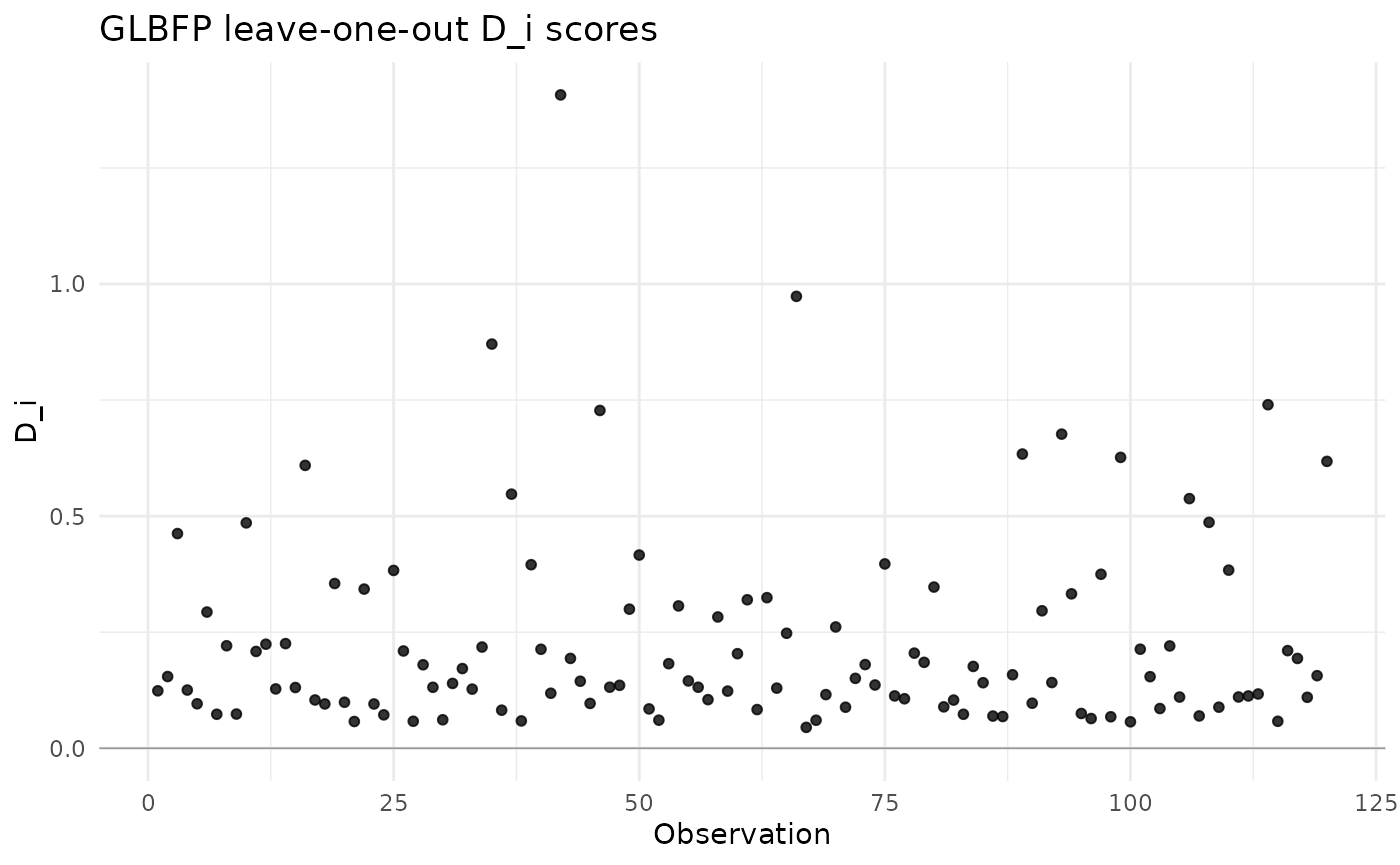

plot(scores, type = "density")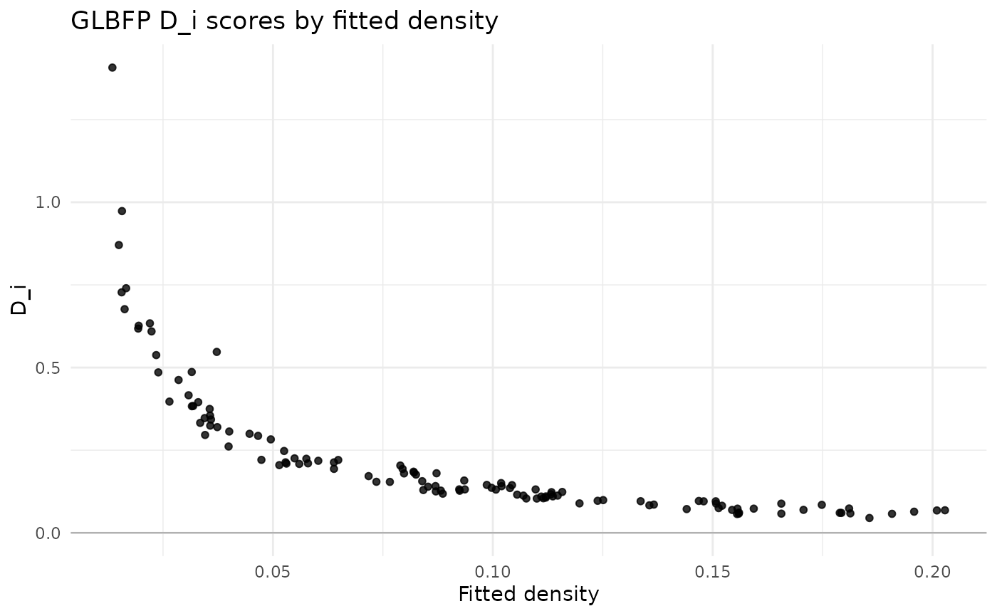

The same interface supports LBFP and ASH.

lbfp_scores <- compute_di(x, b = b, estimator = "LBFP")
ash_scores <- compute_di(x, b = b, m = m, estimator = "ASH")

c(
  LBFP_mean = mean(lbfp_scores$D),
  ASH_mean = mean(ash_scores$D),
  GLBFP_mean = mean(scores$D)
)
#>  LBFP_mean   ASH_mean GLBFP_mean 
#>  0.2481551  0.2654893  0.2296954

Interpretation depends on the chosen estimator, bandwidth and grid. Large positive values indicate observations whose removal substantially decreases their own fitted support under the fixed-grid estimator.