This vignette shows the basic workflow for pointwise and grid-based
density estimation with GLBFP. It is intentionally
practical. For a conceptual map of the full package, see the “Package
overview and workflow map” vignette.
Installation
install.packages("remotes")
remotes::install_github("AurelienNicosiaULaval/GLBFP")Estimate density at one point
The functions ASH(), LBFP(), and
GLBFP() estimate the density at a single point. The data
are supplied as a numeric matrix or data frame with observations in
rows.
x <- matrix(rnorm(300), ncol = 1)
b <- compute_bi_optim(x, m = 1)

fit <- GLBFP(x = 0, data = x, b = b, m = 1)
fit
#> GLBFP Density Estimation:
#> Point: (0)
#> Estimated density: 0.386735
#> Estimated standard error: 0.0838592
#> 95% confidence interval: 0.362643, 0.410827
#> Bandwidths (b): 0.155145
#> Shifts (m): 1
#> Relative grid coordinate (u): 0.916139
Lowercase aliases are also available for interactive workflows. They call the same estimators and keep the uppercase API unchanged.
fit_alias <- glbfp(x = 0, data = x, b = b, m = 1)
identical(fit$estimation, fit_alias$estimation)
#> [1] TRUE
The returned object contains the evaluation point, the estimated
density, the bandwidth, and the shift parameter. For LBFP()
and GLBFP(), uncertainty components are also returned.
names(fit)
#>  [1] "x"            "estimation"   "sd"           "IC"           "b"
#>  [6] "m"            "method"       "dimension"    "u"            "cell_index"
#> [11] "visited"      "prefix_nodes" "prefix_order"
summary(fit)
#> Method: GLBFP
#> Dimension: 1
#> Point: 0
#> Estimation: 0.3867351
#> Standard error: 0.0838592
#> 95% CI: 0.362643259199835, 0.410826868862035
#> Bandwidths (b): 0.155144970240404
#> Shifts (m): 1
#> Relative grid coordinate (u): 0.91613931912711
#> Visited cells: 2
#> Prefix nodes: 2
predict(fit)
#> [1] 0.3867351
Estimate density on a grid
The *_estimate() functions evaluate the same estimator
over a regular grid or a user-supplied set of points.
grid_fit <- GLBFP_estimate(data = x, b = b, m = 1, grid_size = 80)
head(cbind(grid_fit$grid, density = grid_fit$densities))
#>             V1     density
#> [1,] -2.546881 0.085941125
#> [2,] -2.481241 0.067760688
#> [3,] -2.415601 0.049580251
#> [4,] -2.349960 0.031399814
#> [5,] -2.284320 0.017352329
#> [6,] -2.218680 0.008262111
head(as.data.frame(grid_fit))
#>          V1     density          sd    IC_lower   IC_upper visited prefix_nodes
#> 1 -2.546881 0.085941125 0.067942425 0.066422031 0.10546022       2            2
#> 2 -2.481241 0.067760688 0.041194890 0.055925860 0.07959552       2            2
#> 3 -2.415601 0.049580251 0.024146032 0.042643368 0.05651713       2            2
#> 4 -2.349960 0.031399814 0.020860213 0.025406910 0.03739272       2            2
#> 5 -2.284320 0.017352329 0.016030533 0.012746937 0.02195772       1            2
#> 6 -2.218680 0.008262111 0.009668979 0.005484322 0.01103990       1            2
For one-dimensional grids, the plot method returns a
ggplot2 object.
plot(grid_fit)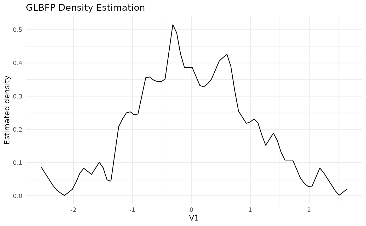
Using the included data
The ashua data contain daily flow and level observations
for the Ashuapmushuan river. The example below uses a small grid so the
vignette remains fast.
data("ashua")

river_data <- ashua[, c("flow", "level")]
b2 <- c(8, 0.4)
x0 <- c(mean(river_data$flow), mean(river_data$level))

fit2 <- GLBFP(x = x0, data = river_data, b = b2, m = c(1, 1))
fit2
#> GLBFP Density Estimation:
#> Point: (249.0230, 30.4197)
#> Estimated density: 0.00377442
#> Estimated standard error: 0.000316735
#> 95% confidence interval: 0.00376918, 0.00377966
#> Bandwidths (b): 8.0, 0.4
#> Shifts (m): 1, 1
#> Relative grid coordinate (u): 0.690325, 0.224216

grid_fit2 <- GLBFP_estimate(
  data = river_data,
  b = b2,
  m = c(1, 1),
  grid_size = 15
)

plot(grid_fit2, contour = TRUE)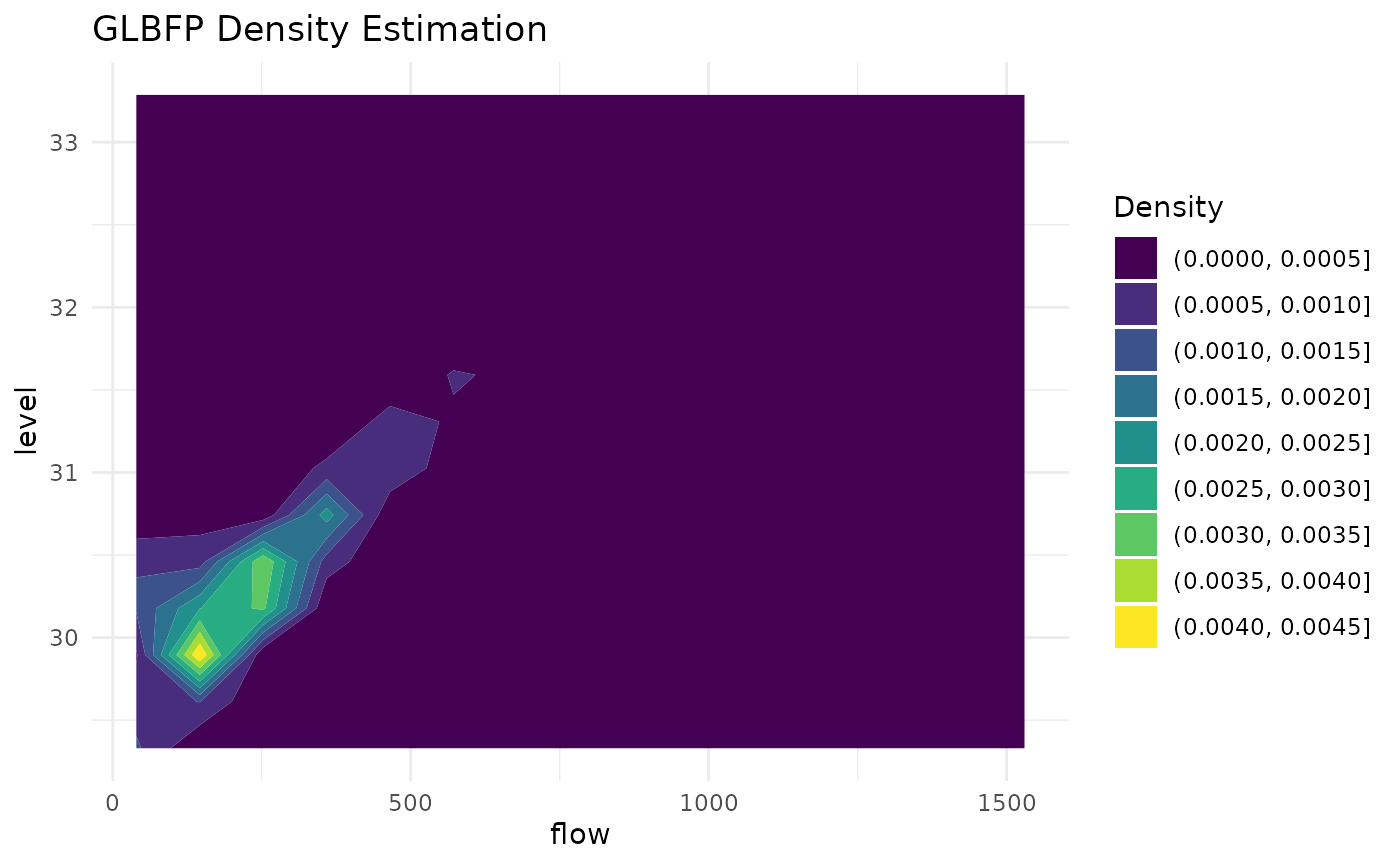
Leave-one-out scores
The function compute_Di() computes fixed-grid
leave-one-out self-support scores. These scores are useful for
diagnosing observations that receive little support from the fitted grid
estimator.
scores <- compute_Di(
  river_data,
  b = b2,
  m = c(1, 1),
  estimator = "GLBFP"
)

summary(scores)
#> D_i score summary
#> Method: GLBFP
#> Observations: 4389
#> Dimension: 2
#> D_i quantiles:
#>          0%         25%         50%         75%        100%
#> 0.002067332 0.009058091 0.012657309 0.029337142 1.000000000
#> D_i mean: 0.04055607
#> Missing D_i: 21
#> Density range: 0 to 0.0107203911768057
#> Median visited cells: 4
#> Median prefix nodes: 6
head(as.data.frame(scores))
#>   observation           D  D_positive     density density_loo self_weight
#> 1           1 0.008458264 0.008458264 0.004114824 0.004080019   0.5018750
#> 2           2 0.010079869 0.010079869 0.004156231 0.004114337   0.6015625
#> 3           3 0.008665307 0.008665307 0.004239247 0.004202513   0.5293750
#> 4           4 0.008332855 0.008332855 0.004258293 0.004222809   0.5118750
#> 5           5 0.007595790 0.007595790 0.004437585 0.004403878   0.4875000
#> 6           6 0.008239098 0.008239098 0.004360644 0.004324716   0.5184375
#>   visited prefix_nodes
#> 1       4            6
#> 2       4            6
#> 3       4            6
#> 4       4            6
#> 5       4            6
#> 6       4            6
plot(scores)
#> Warning: Removed 21 rows containing missing values or values outside the scale range
#> (`geom_point()`).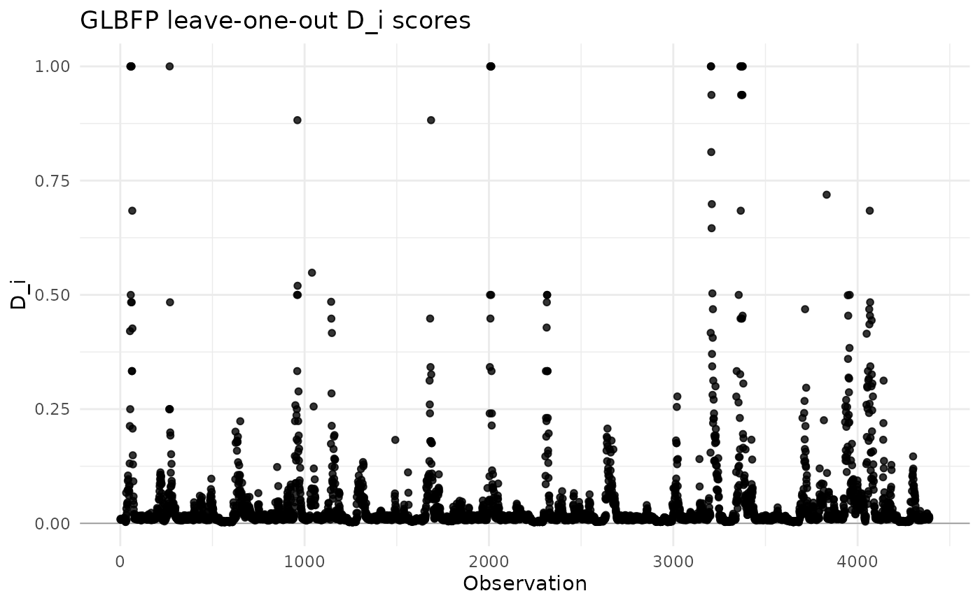
Input expectations
The package expects finite numeric data. Missing values should be
removed or imputed before estimation. Constant data require explicit
non-degenerate min_vals and max_vals bounds
because a density estimator for continuous data needs a positive
evaluation range.
Where to go next
After this vignette:
- read “Brief methodological background” for the statistical context;
- read “Choosing between ASH, LBFP and GLBFP” when comparing estimators;
- read “Two-dimensional density estimation” for 2D workflows;
- read “Sparse-prefix computation” and “Leave-one-out D_i diagnostics” for implementation diagnostics.