Two-dimensional density estimation • GLBFP

This vignette illustrates two-dimensional density estimation and visualization. It complements the estimator-choice vignette by focusing on the 2D workflow.

library(GLBFP)

Simulated example

The example uses a small reproducible mixture so the vignette remains quick to build.

n <- 250
group <- rbinom(n, size = 1, prob = 0.5)

x <- cbind(
  rnorm(n, mean = ifelse(group == 1, -1.2, 1.2), sd = 0.7),
  rnorm(n, mean = ifelse(group == 1, 1.0, -1.0), sd = 0.8)
)

colnames(x) <- c("x1", "x2")

b <- compute_bi_optim(x, m = c(1, 1))
b
#> [1] 0.3210361 0.3159536

Pointwise estimation

x0 <- c(0, 0)

ash_fit <- ash(x0, x, b = b, m = c(1, 1))
lbfp_fit <- lbfp(x0, x, b = b)
glbfp_fit <- glbfp(x0, x, b = b, m = c(1, 1))

c(
  ASH = ash_fit$estimation,
  LBFP = lbfp_fit$estimation,
  GLBFP = glbfp_fit$estimation
)
#>        ASH       LBFP      GLBFP 
#> 0.03943508 0.01941260 0.01941260

Grid estimation

grid_fit <- glbfp_estimate(x, b = b, m = c(1, 1), grid_size = 20)
summary(grid_fit)
#> Method: GLBFP 
#> Dimension: 2 
#> Grid points: 400 
#> Grid type: rectangular 
#> Grid dimensions: 20 x 20 
#> Bandwidths (b): 0.321036127107069, 0.315953610723842 
#> Shifts (m): 1, 1 
#> Density range: 0 to 0.210331281836707 
#> Density quartiles: 0, 0.00348642703612875, 0.0356905349965338 
#> Density median: 0.003486427 
#> Density mean: 0.02480127 
#> Zero densities: 188 
#> Standard error median: 0.007210991 
#> Median visited cells: 1 
#> Median prefix nodes: 6
head(as.data.frame(grid_fit))
#>          x1        x2 density sd IC_lower IC_upper visited prefix_nodes
#> 1 -2.974658 -2.888704       0  0        0        0       0            6
#> 2 -2.657723 -2.888704       0  0        0        0       0            6
#> 3 -2.340789 -2.888704       0  0        0        0       0            6
#> 4 -2.023855 -2.888704       0  0        0        0       0            6
#> 5 -1.706920 -2.888704       0  0        0        0       0            6
#> 6 -1.389986 -2.888704       0  0        0        0       0            6

Visualization

For two-dimensional regular grids, contour = TRUE returns a static ggplot2 contour plot.

plot(grid_fit, contour = TRUE)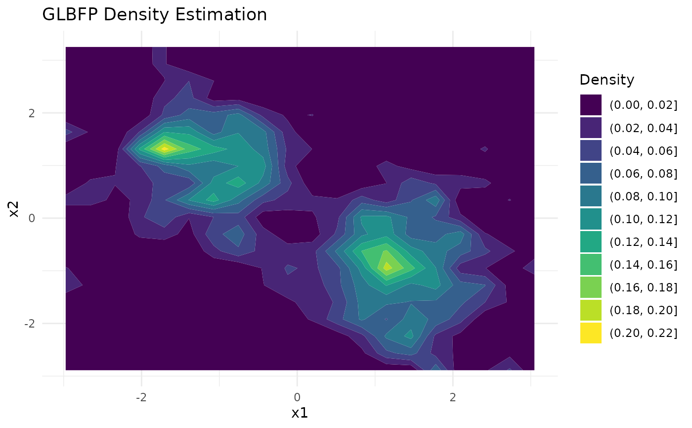

With contour = FALSE, the plot method returns an interactive plotly surface. This is useful for exploration. Static contours are usually easier to reproduce in manuscripts.

surface <- plot(grid_fit, contour = FALSE)
surface

Computational note

The number of evaluation points grows quickly with grid_size in two dimensions. For manuscript figures, start with a moderate grid and increase it only after confirming that the visual conclusions are stable.