LBFP density estimation on a grid

Computes LBFP density estimates on a regular or user-supplied grid.

Usage

LBFP_estimate(
  data,
  b = compute_bi_optim(data, m = rep(1, ncol(data))),
  grid_size = 20,
  grid_points = NULL,
  min_vals = apply(data, 2, min),
  max_vals = apply(data, 2, max)
)

# S3 method for class 'LBFP_estimate'
print(x, ...)

# S3 method for class 'LBFP_estimate'
plot(x, contour = FALSE, ...)

Arguments

data: Numeric matrix or data frame of observations (n x d).
b: Positive numeric vector of bandwidths (length d).
grid_size: Integer number of grid points per dimension when grid_points = NULL.
grid_points: Optional matrix/data frame of explicit evaluation points.
min_vals: Numeric vector of lower grid bounds (length d).
max_vals: Numeric vector of upper grid bounds (length d).
x: Object returned by LBFP_estimate().
...: Additional arguments (unused).
contour: If TRUE, draw a contour-like 2D representation for 2D data.

Value

A list with class c("glbfp_grid", "LBFP_estimate") containing grid coordinates, densities, uncertainty estimates, and grid metadata.

Details

When grid_points is NULL, a regular grid is constructed from min_vals to max_vals. Custom grids may be irregular; in that case plotting uses point or scatter representations instead of a surface.

Methods (by generic)

print(LBFP_estimate): Print method for object of class "LBFP_estimate".
plot(LBFP_estimate): Plot method for object of class "LBFP_estimate".

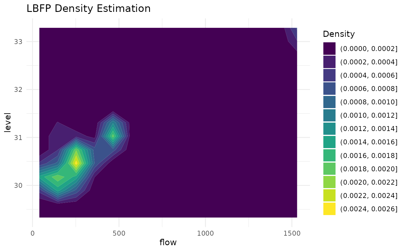
Examples

b <- c(0.5, 0.5)
out <- LBFP_estimate(ashua[, -3], b = b, grid_size = 15)
out
#> LBFP Density Estimation on Grid:
#> Grid points: 225 
#> Dimensions: 2 
#> Grid type: rectangular 
#> Density range: 0.00000000, 0.00250857 
#> Bandwidths (b): 0.5, 0.5 
#> Shifts (m): LBFP 
#> Median visited cells: 0 
#> Median prefix nodes: 6 
plot(out, contour = TRUE)