Comparative validation notes

Scope

This article records lightweight comparative checks for ggcircular. It is a pkgdown article rather than a CRAN vignette because it may grow into a longer validation document for a software paper.

The focus is practical agreement on core quantities:

1. circular mean direction;
2. mean resultant length;
3. axial summaries;
4. von Mises simulation and mixture diagnostics;
5. timing and memory proxies for common plotting workflows.

library(ggplot2)
library(dplyr)
#> 
#> Attaching package: 'dplyr'
#> The following objects are masked from 'package:stats':
#> 
#>     filter, lag
#> The following objects are masked from 'package:base':
#> 
#>     intersect, setdiff, setequal, union
library(ggcircular)

Optional package availability

comparison_packages <- c("circular", "CircStats", "NPCirc", "Directional")

tibble(
  package = comparison_packages,
  available = vapply(comparison_packages, requireNamespace, logical(1), quietly = TRUE)
)
#> # A tibble: 4 × 2
#>   package     available
#>   <chr>       <lgl>    
#> 1 circular    TRUE     
#> 2 CircStats   FALSE    
#> 3 NPCirc      FALSE    
#> 4 Directional FALSE

Boundary behaviour

boundary <- tibble(theta = c(0.02, 0.04, 2 * pi - 0.03, 2 * pi - 0.01))

boundary |>
  summarise(
    arithmetic_mean = mean(theta),
    circular_mean = mean_direction(theta),
    Rbar = mean_resultant_length(theta)
  )
#> # A tibble: 1 × 3
#>   arithmetic_mean circular_mean  Rbar
#>             <dbl>         <dbl> <dbl>
#> 1            3.15       0.00500 1.000

ggplot(boundary, aes(x = theta)) +
  geom_rose(bins = 16, alpha = 0.7) +
  geom_mean_direction(colour = "#123C4A", linewidth = 1) +
  scale_x_circular_degrees() +
  coord_circular() +
  theme_circular()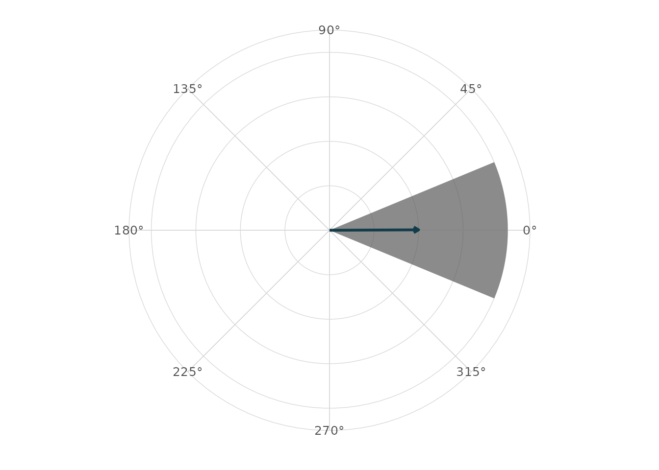

Comparison with circular when available

if (requireNamespace("circular", quietly = TRUE)) {
  x <- c(rnorm(120, 0.5, 0.25), rnorm(120, 5.8, 0.25))
  x <- normalize_angle(x)

  circular_x <- circular::circular(x)

  tibble(
    statistic = c("mean", "Rbar"),
    ggcircular = c(mean_direction(x), mean_resultant_length(x)),
    circular = c(
      as.numeric(circular::mean.circular(circular_x)),
      as.numeric(circular::rho.circular(circular_x))
    ),
    absolute_difference = abs(ggcircular - circular)
  )
}
#> # A tibble: 2 × 4
#>   statistic ggcircular circular absolute_difference
#>   <chr>          <dbl>    <dbl>               <dbl>
#> 1 mean          0.0196   0.0196            1.53e-16
#> 2 Rbar          0.855    0.855             0    

Uniform data

uniform_angles <- seq(0, 2 * pi, length.out = 181)[-181]

tibble(
  mean = mean_direction(uniform_angles),
  Rbar = mean_resultant_length(uniform_angles),
  rayleigh_p_value = rayleigh_test(uniform_angles)$p.value
)
#> # A tibble: 1 × 3
#>    mean     Rbar rayleigh_p_value
#>   <dbl>    <dbl>            <dbl>
#> 1    NA 1.90e-17                1

Axial data

axial_example <- tibble(
  orientation = normalize_angle(c(
    rnorm(60, 0.1, 0.08),
    rnorm(60, pi + 0.1, 0.08)
  ))
)

axial_example |>
  summarise(
    directional_Rbar = mean_resultant_length(orientation),
    axial_Rbar = mean_resultant_length(orientation, axial = TRUE),
    axial_mean = mean_direction(orientation, axial = TRUE)
  )
#> # A tibble: 1 × 3
#>   directional_Rbar axial_Rbar axial_mean
#>              <dbl>      <dbl>      <dbl>
#> 1          0.00536      0.986      0.112

ggplot(axial_example, aes(x = orientation)) +
  geom_rose(bins = 18, axial = TRUE, alpha = 0.75) +
  geom_mean_direction(axial = TRUE, colour = "#123C4A", linewidth = 1) +
  scale_x_circular_degrees(limits = c(0, pi)) +
  coord_circular() +
  theme_circular()
#> Warning: Removed 61 rows containing non-finite outside the scale range
#> (`stat_rose()`).
#> Warning: Removed 61 rows containing non-finite outside the scale range
#> (`stat_mean_direction()`).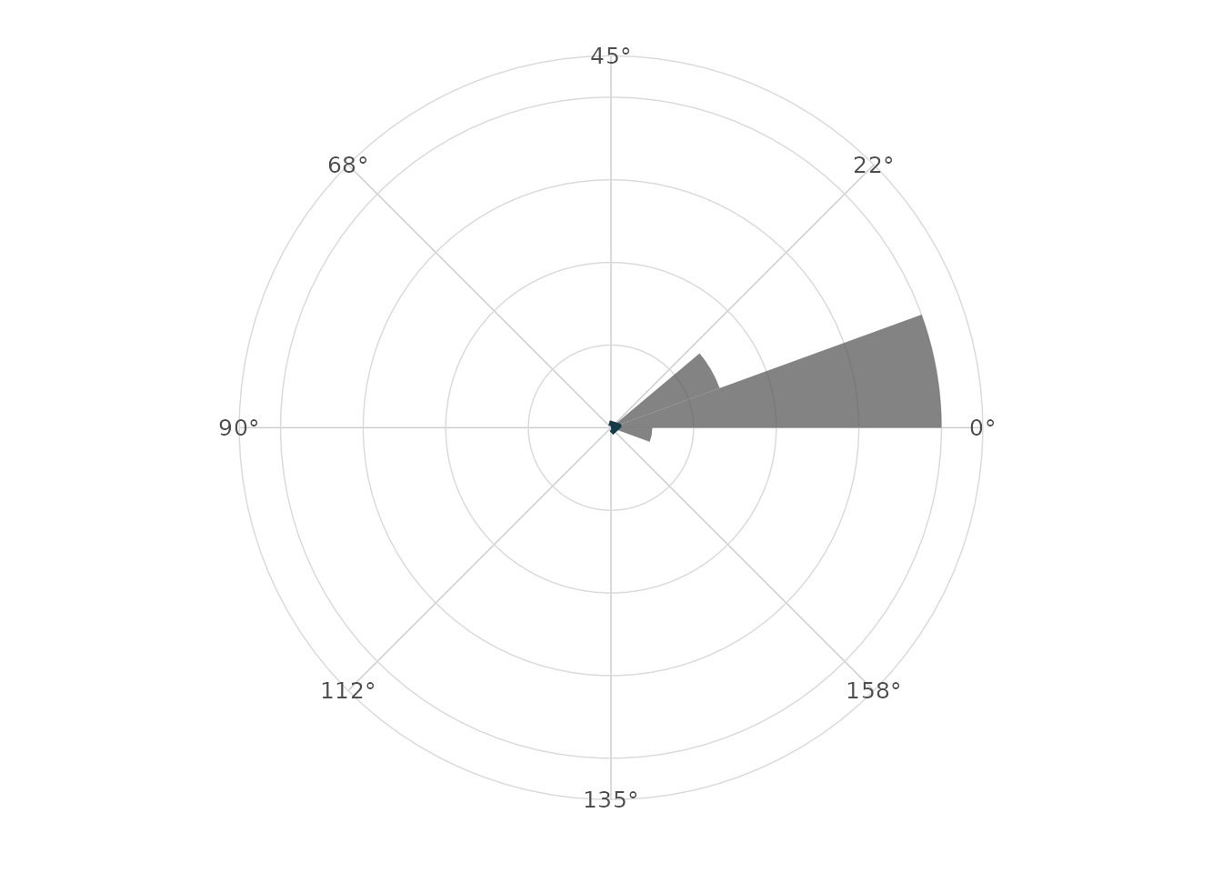

Bimodal mixture

set.seed(2026)
bimodal <- normalize_angle(c(rnorm(100, 0.8, 0.2), rnorm(100, 4.1, 0.25)))
fit <- fit_vonmises_mixture(bimodal, k = 2, nstart = 5, seed = 2026)

tidy_circular(fit)
#> # A tibble: 2 × 4
#>   component proportion    mu kappa
#>       <int>      <dbl> <dbl> <dbl>
#> 1         1      0.500 0.780  25.6
#> 2         2      0.500 4.13   18.1
glance_circular(fit)
#> # A tibble: 1 × 12
#>       n components logLik   AIC   BIC iterations converged nstart start_id
#>   <int>      <int>  <dbl> <dbl> <dbl>      <int> <lgl>      <int>    <int>
#> 1   200          2  -118.  246.  262.          4 TRUE           5        1
#> # ℹ 3 more variables: empty_components <int>, kappa_max <dbl>, axial <lgl>

ggplot(tibble(theta = bimodal), aes(x = theta)) +
  geom_rose(aes(y = after_stat(density)), bins = 24, alpha = 0.45) +
  stat_vonmises_mixture(fit = fit, linewidth = 1) +
  scale_x_circular_degrees() +
  coord_circular() +
  theme_circular()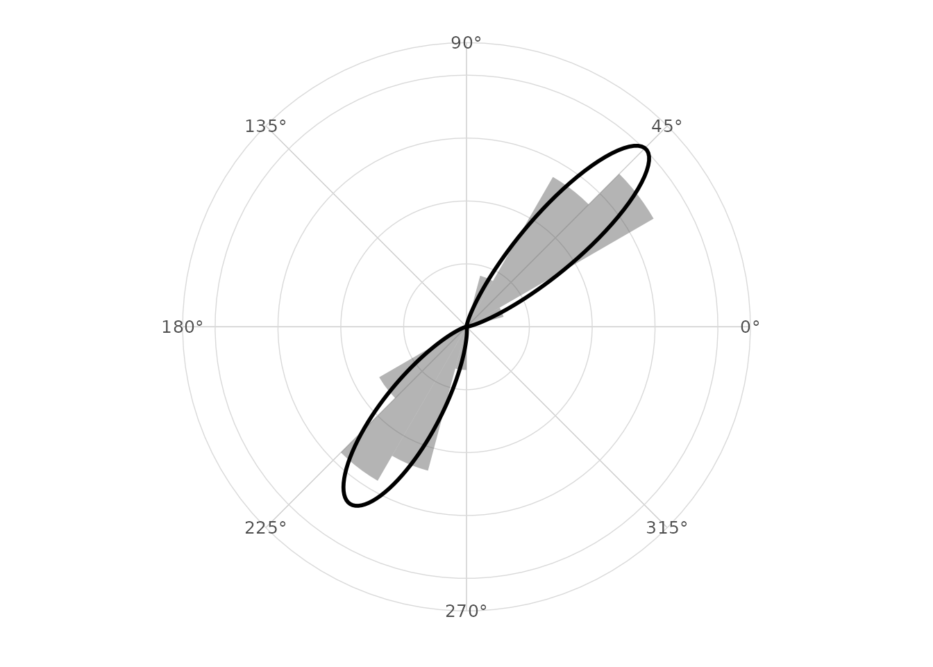

Timing proxy

set.seed(1)
timing_data <- normalize_angle(rnorm(1000, 1, 0.7))

system.time({
  density_tbl <- ggplot_build(
    ggplot(tibble(theta = timing_data), aes(x = theta)) +
      stat_circular_density(n = 256)
  )$data[[1]]
})
#>    user  system elapsed 
#>   0.041   0.001   0.042

density_tbl |>
  summarise(n_grid = n(), density_min = min(density), density_max = max(density))
#>   n_grid density_min density_max
#> 1    256  0.01047087   0.3970394

Applied examples to keep validating

The main validation examples for an article should remain reproducible and small:

1. wind direction with compass bearings;
2. animal movement turn angles by state;
3. axial orientation data;
4. circular residual diagnostics from angular regression;
5. posterior angular draws when posterior is installed.

These examples are already represented in the package datasets and focused articles. The next validation pass should add formal numerical comparisons for packages that are installed in the full-suggests CI profile.