![]()
![]()
![]()
![]()

![]()
![]()
![]()
ggcircular is a ggplot2 extension for circular, axial and directional data. It provides layers, scales, coordinate helpers, summaries and diagnostics for angles measured on a periodic scale.
The package is designed for exploratory graphics, teaching examples and reproducible statistical workflows involving directions, bearings, orientations, times of day, turn angles and other circular measurements.
Part of the research ecosystem
This repository is part of Aurélien Nicosia’s open research and teaching ecosystem in computational statistics, scientific R software, reproducible data science and statistical education.
- Research Lab: https://aureliennicosiaulaval.github.io/web_site/research-lab.html
- GitHub profile: https://github.com/AurelienNicosiaULaval
- Related projects:
CircularRegression,donnees-bleues
Installation
Development version
Install the development version from GitHub:
install.packages("remotes")
remotes::install_github("AurelienNicosiaULaval/ggcircular")
Or clone with SSH and install locally:
Quick Start
wind_directions |>
  filter(season == "winter") |>
  ggplot(aes(x = direction)) +
  geom_rose(aes(y = after_stat(density), fill = after_stat(density)), bins = 24, alpha = 0.78) +
  geom_circular_density(linewidth = 1.1, colour = "#123C4A") +
  geom_mean_direction(length = "resultant", colour = "#E4572E", linewidth = 1.1) +
  scale_x_circular_compass() +
  coord_circular(zero = "north", direction = "clockwise") +
  labs(fill = "density", title = "Winter wind directions") +
  theme_circular()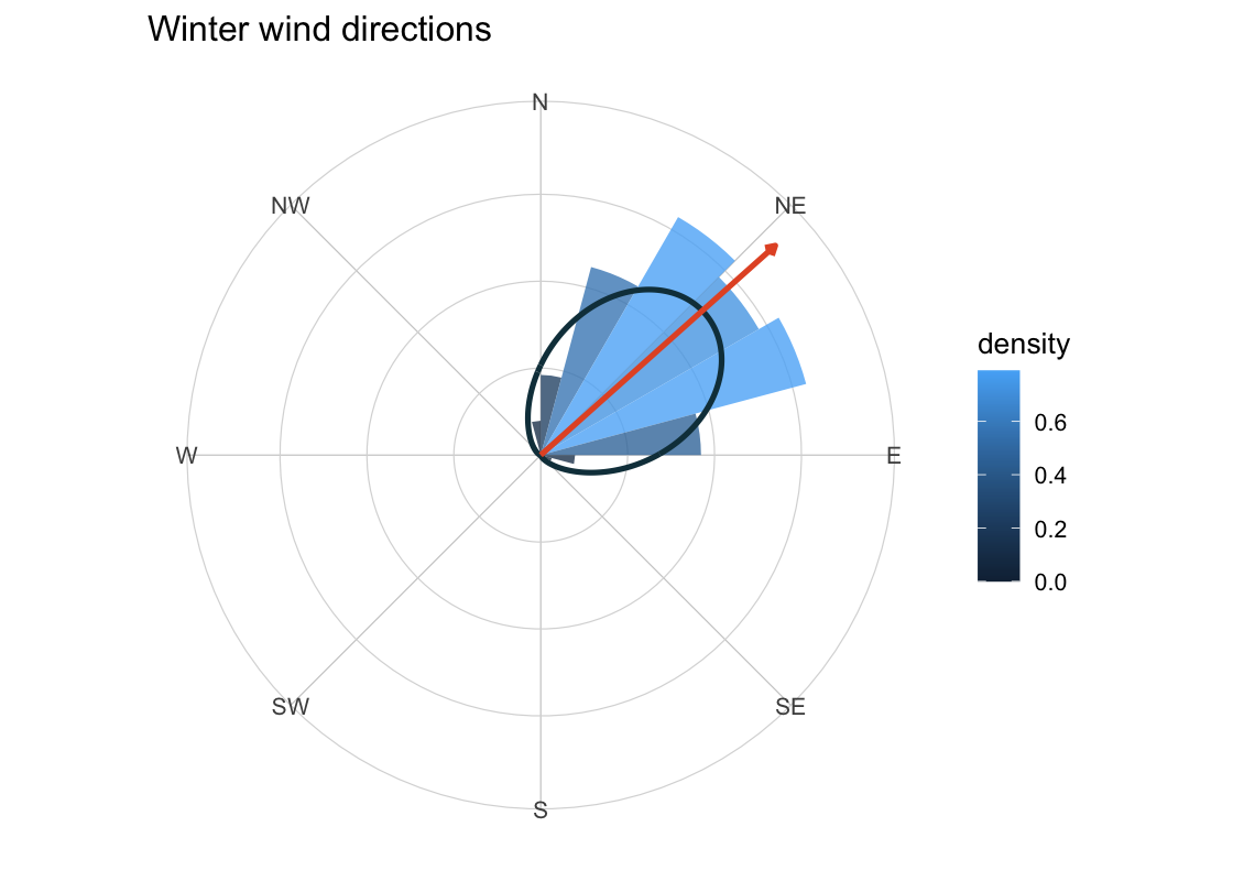
What It Does
| Workflow | Main helpers |
|---|---|
| Rose diagrams and circular histograms |
geom_rose(), stat_rose()
|
| Circular density estimation |
geom_circular_density(), stat_circular_density()
|
| Mean direction and concentration |
geom_mean_direction(), circular_summary(), estimate_kappa()
|
| Circular confidence intervals and tests |
circular_mean_ci(), rayleigh_test(), watson_williams_test(), stat_circular_test()
|
| Axial orientations modulo pi |
axial = TRUE in summaries and layers |
| Theoretical circular distributions |
stat_vonmises(), stat_wrapped_normal(), stat_uniform_circular()
|
| Mixtures of von Mises components |
fit_vonmises_mixture(), stat_vonmises_mixture()
|
| Movement and state-angle graphics |
mutate_directional_features(), geom_direction_arrow(), plot_state_angles()
|
| Angular model diagnostics |
circular_residuals(), circular_model_diagnostics(), autoplot() methods |
| Spherical and posterior helpers |
spherical_summary(), as_circular_draws(), summarise_circular_draws()
|
Design Principles
- Angles are stored and computed in radians.
- Scales handle display labels in radians, degrees, hours or compass labels.
- Directional data use period
2 * pi. - Axial data use period
pithroughaxial = TRUE. - Heavy packages remain optional and are accessed with explicit availability checks.
- Outputs are standard
ggplotobjects, tibbles or familiar test objects.
Conventions for Directions and Bearings
The default mathematical convention is zero = "east" with angles increasing counterclockwise. This matches the usual unit circle.
Compass bearings use zero = "north" with angles increasing clockwise. Use scale_x_circular_compass() together with coord_circular(zero = "north", direction = "clockwise") for bearing-like data such as wind direction or movement headings.
Axial data, such as unoriented lines, are different again: 0 and pi represent the same orientation. Use axial = TRUE in summaries and layers for these data.
Summaries
circular_summary() respects existing dplyr groups and returns mean direction, resultant length, circular variance, circular standard deviation and an estimated von Mises concentration parameter. estimate_kappa() is a descriptive piecewise approximation from the sample resultant length, not a full inferential fit.
wind_directions |>
  circular_summary(direction, season) |>
  mutate(
    mean_degrees = round(rad_to_deg(mean), 1),
    Rbar = round(Rbar, 3),
    kappa = round(kappa, 2)
  ) |>
  select(season, n, mean_degrees, Rbar, kappa)
#> # A tibble: 4 × 5
#>   season     n mean_degrees  Rbar kappa
#>   <chr>  <int>        <dbl> <dbl> <dbl>
#> 1 fall     131        310.  0.811  3
#> 2 spring   115        135.  0.802  2.89
#> 3 summer   138        223.  0.87   4.15
#> 4 winter   116         48.2 0.904  5.52
Axial Data
Axial observations identify opposite directions. For example, an orientation of 0 radians is equivalent to an orientation of pi radians. Use axial = TRUE to compute and display these data modulo pi.
ggplot(axial_orientations, aes(x = orientation, fill = group)) +
  geom_rose(bins = 18, axial = TRUE, alpha = 0.72) +
  geom_mean_direction(axial = TRUE, colour = "#123C4A", linewidth = 1) +
  scale_x_circular_degrees(limits = c(0, pi)) +
  coord_circular() +
  facet_wrap(~ group) +
  theme_circular()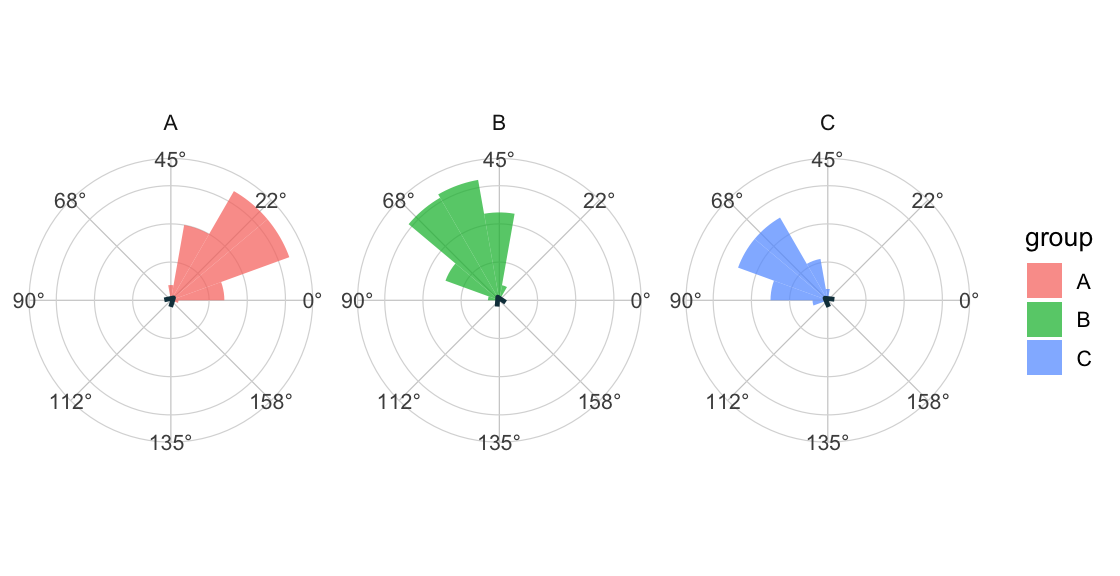
Directional Movement
ggcircular includes helpers for bearings, turn angles and state-specific angular distributions.
animal_steps |>
  filter(!is.na(turn_angle)) |>
  ggplot(aes(x = turn_angle, fill = state)) +
  geom_rose(bins = 24, alpha = 0.72) +
  geom_mean_direction(colour = "#123C4A", linewidth = 1) +
  scale_x_circular_degrees(
    breaks = deg_to_rad(c(0, 90, 180, 270)),
    labels = c("0", "90", "180", "270")
  ) +
  coord_circular() +
  facet_wrap(~ state) +
  theme_circular()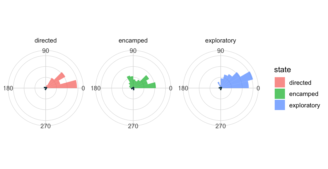
Mixtures of von Mises Distributions
Finite mixtures are fitted with an expectation-maximization routine and can be drawn directly on top of empirical rose diagrams. These fits are descriptive and depend on initialization, so use seed, nstart and diagnostic output when the mixture is substantively important.
set.seed(2026)

fit_mix <- fit_vonmises_mixture(
  wind_directions$direction,
  k = 2,
  init = "spaced",
  nstart = 3,
  seed = 2026
)

ggplot(wind_directions, aes(x = direction)) +
  geom_rose(aes(y = after_stat(density)), bins = 24, alpha = 0.42) +
  stat_vonmises_mixture(fit = fit_mix, linewidth = 1.2, colour = "#123C4A") +
  scale_x_circular_degrees() +
  coord_circular() +
  theme_circular()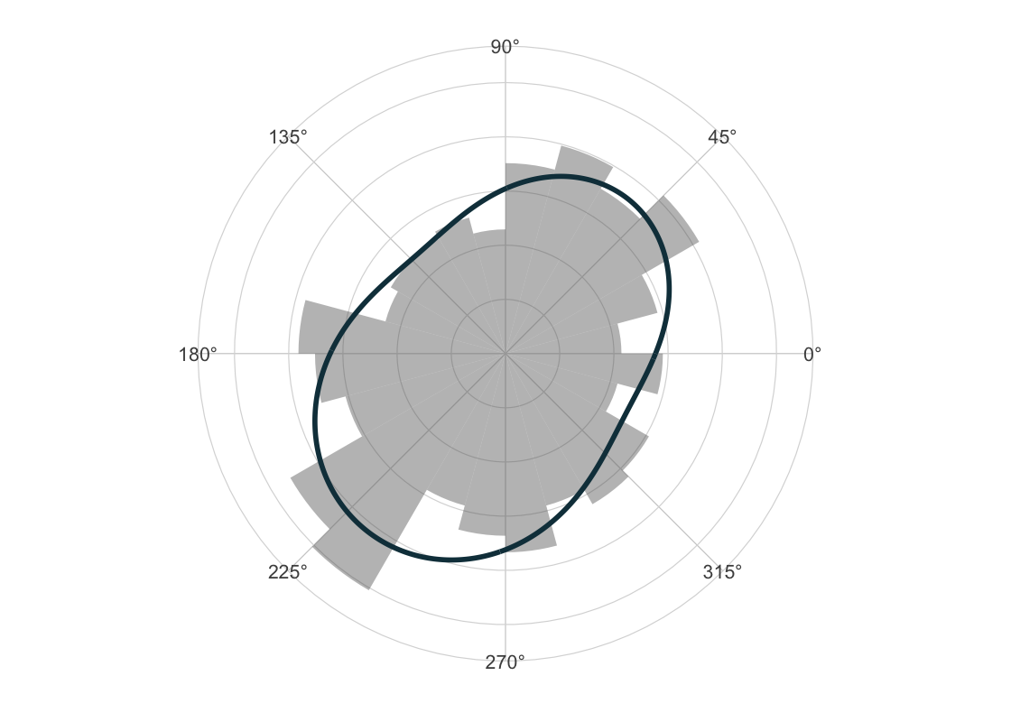
tidy_circular(fit_mix) |>
  mutate(
    mu_degrees = round(rad_to_deg(mu), 1),
    kappa = round(kappa, 2),
    proportion = round(proportion, 3)
  ) |>
  select(component, proportion, mu_degrees, kappa)
#> # A tibble: 2 × 4
#>   component proportion mu_degrees kappa
#>       <int>      <dbl>      <dbl> <dbl>
#> 1         1      0.328       51.6  1.45
#> 2         2      0.672      232.   0.77
Tests and Intervals
circular_mean_ci(
  wind_directions$direction,
  method = "bootstrap",
  R = 399,
  seed = 2026
) |>
  mutate(across(c(mean, lower, upper), rad_to_deg))
#> # A tibble: 1 × 7
#>    mean lower upper level method        n   Rbar
#>   <dbl> <dbl> <dbl> <dbl> <chr>     <int>  <dbl>
#> 1  235.  139.  354.  0.95 bootstrap   500 0.0494
rayleigh <- rayleigh_test(wind_directions$direction)

tibble::tibble(
  statistic = unname(rayleigh$statistic),
  n = unname(rayleigh$parameter),
  p_value = rayleigh$p.value,
  method = rayleigh$method
)
#> # A tibble: 1 × 4
#>   statistic     n p_value method
#>       <dbl> <int>   <dbl> <chr>
#> 1      1.22   500   0.295 Rayleigh test of circular uniformity
Optional Model Integrations
The package keeps heavier modeling ecosystems in Suggests. When available, these integrations add diagnostics without making them hard dependencies.
fit <- CircularRegression::consensus(direction ~ speed, data = wind_directions)

circular_model_diagnostics(fit)

autoplot(fit, type = "residuals_density")
autoplot(fit, type = "fitted_observed")
Optional helpers currently target:
-
CircularRegression-style angular, consensus and two-step objects through S3 class support. -
momentuHMMstate probabilities and Viterbi states. -
posteriordraw objects throughposterior::as_draws_df(). -
circulartests when classical circular test implementations are available.
Experimental Features
The following pieces are intentionally available but still experimental:
- angular model diagnostics for optional external model classes;
- finite mixtures of von Mises distributions;
-
momentuHMMstate-angle adapters; - spherical summaries and posterior draw helpers.
Experimental functions are documented and tested, but their return columns may still evolve as validation reveals better public contracts.
Statistical Limitations
ggcircular is primarily a visualization and diagnostics package. It does not replace specialist inference workflows for circular statistics.
- The automatic density bandwidth is a simple heuristic.
-
circular_mean_ci()is unreliable when the mean resultant length is close to zero because the mean direction is weakly identified. -
rayleigh_test()is mainly sensitive to unimodal departures from uniformity. -
watson_williams_test()relies on strong assumptions about group concentration and uses the optionalcircularimplementation. - Multimodal data should usually be inspected with density or mixture graphics, not summarized only by one mean direction.
CRAN Status
ggcircular is available from CRAN at https://CRAN.R-project.org/package=ggcircular. The CRAN page lists version 0.1.0, published 2026-06-04, source archives, binaries, vignettes and check results.
The development workflow continues to include:
-
R CMD check --as-cranon the final source tarball; -
--run-donttestchecks; - hard-dependency checks with
_R_CHECK_FORCE_SUGGESTS_=false; - full-suggests checks when optional packages are available;
- Linux R-devel, Linux R-release, macOS R-release and Windows R-release checks;
- vignette build timing and source tarball size checks.
Longer articles are built for pkgdown and excluded from the CRAN tarball.
Citation
To cite ggcircular from R, use:
citation("ggcircular")Citation metadata is also provided in inst/CITATION.
Contributing and Support
Contributions are welcome through focused GitHub issues and pull requests. See CONTRIBUTING.md, SUPPORT.md and CODE_OF_CONDUCT.md for contribution, support and conduct guidelines.
Development Status
ggcircular is currently experimental. The public API is usable, tested and documented, but may still evolve as more angular model classes and validation cases are added.
Current checks:
- Local
devtools::test()passes. - Local
devtools::check(document = FALSE, args = "--as-cran", build_args = "--no-manual")is used before release commits. - GitHub Actions runs hard-dependency checks with
_R_CHECK_FORCE_SUGGESTS_=falseand full-suggests checks when optional packages are available. - GitHub Actions includes Linux R-devel plus Linux, macOS and Windows R-release.
-
pkgdownbuilds and publishes the website frommain.
References
- Fisher, N. I. (1993). Statistical Analysis of Circular Data. Cambridge University Press.
- Jammalamadaka, S. R., and Sengupta, A. (2001). Topics in Circular Statistics. World Scientific.
- Pewsey, A., Neuhäuser, M., and Ruxton, G. D. (2013). Circular Statistics in R. Oxford University Press.
- Wickham, H. (2016). ggplot2: Elegant Graphics for Data Analysis. Springer.