Overview
ggcircular extends ggplot2 for circular,
axial and directional data. This vignette gives a complete first tour of
the package: angle conventions, rose diagrams, circular densities, mean
directions, uncertainty, axial data, movement data, mixtures of von
Mises distributions and model diagnostics.
Not on CRAN yet
ggcircular is not on CRAN yet. The package is being
stabilized for a first CRAN submission; install the development version
from GitHub for now.
Why circular data are different
Circular observations live on a periodic scale. In radians,
0 and 2 * pi represent the same direction.
This means that linear tools can fail near the boundary.
boundary_angles <- tibble(
  theta = c(0.05, 0.10, 2 * pi - 0.10, 2 * pi - 0.05)
)

boundary_angles |>
  summarise(
    arithmetic_mean = mean(theta),
    circular_mean = mean_direction(theta),
    Rbar = mean_resultant_length(theta)
  )
#> # A tibble: 1 × 3
#>   arithmetic_mean circular_mean  Rbar
#>             <dbl>         <dbl> <dbl>
#> 1            3.14             0 0.997
The arithmetic mean is near pi, even though the
observations are concentrated near zero. The circular mean uses sine and
cosine components, so it respects the periodic scale.
Data included in the package
The package ships with four simulated datasets. They are small enough for examples and large enough to show realistic grouped workflows.
glimpse(wind_directions)
#> Rows: 500
#> Columns: 4
#> $ station   <chr> "station_C", "station_B", "station_B", "station_B", "station…
#> $ direction <dbl> 3.61399414, 0.51640381, 3.18127144, 2.81398312, 3.48203785, …
#> $ speed     <dbl> 8.344303, 21.651462, 18.502725, 17.959547, 14.707662, 23.812…
#> $ season    <chr> "summer", "winter", "summer", "spring", "summer", "winter", …
glimpse(animal_steps)
#> Rows: 600
#> Columns: 8
#> $ id          <chr> "animal_1", "animal_1", "animal_1", "animal_1", "animal_1"…
#> $ time        <int> 1, 2, 3, 4, 5, 6, 7, 8, 9, 10, 11, 12, 13, 14, 15, 16, 17,…
#> $ x           <dbl> -2.0936857, -1.2574724, 1.3703509, 1.8277511, 3.1477115, 3…
#> $ y           <dbl> -2.206504, -4.007244, -5.236538, -5.303458, -5.208255, -5.…
#> $ step_length <dbl> NA, 1.9854255, 2.9011413, 0.4622696, 1.3233892, 0.1811402,…
#> $ bearing     <dbl> NA, 5.14713037, 5.84562829, 6.13791093, 0.07200064, 0.1664…
#> $ turn_angle  <dbl> NA, NA, 0.69849792, 0.29228264, 0.21727502, 0.09441297, -2…
#> $ state       <chr> "exploratory", "directed", "exploratory", "encamped", "dir…
glimpse(hourly_activity)
#> Rows: 240
#> Columns: 5
#> $ id       <chr> "id_1", "id_1", "id_1", "id_1", "id_1", "id_1", "id_1", "id_1…
#> $ hour     <int> 0, 1, 2, 3, 4, 5, 6, 7, 8, 9, 10, 11, 12, 13, 14, 15, 16, 17,…
#> $ angle    <dbl> 0.0000000, 0.2617994, 0.5235988, 0.7853982, 1.0471976, 1.3089…
#> $ activity <dbl> 0.7068110, 0.9307937, 0.8454886, 1.1279882, 1.2763149, 1.8896…
#> $ group    <chr> "control", "control", "control", "control", "control", "contr…
glimpse(axial_orientations)
#> Rows: 300
#> Columns: 3
#> $ sample      <chr> "sample_4", "sample_9", "sample_1", "sample_3", "sample_7"…
#> $ orientation <dbl> 0.33720049, 1.29682693, 0.90355276, 1.08422434, 1.01917603…
#> $ group       <chr> "A", "C", "B", "C", "C", "C", "B", "C", "A", "A", "B", "A"…
wind_directions |>
  count(season, station)
#> # A tibble: 16 × 3
#>    season station       n
#>    <chr>  <chr>     <int>
#>  1 fall   station_A    40
#>  2 fall   station_B    31
#>  3 fall   station_C    27
#>  4 fall   station_D    33
#>  5 spring station_A    32
#>  6 spring station_B    26
#>  7 spring station_C    31
#>  8 spring station_D    26
#>  9 summer station_A    21
#> 10 summer station_B    36
#> 11 summer station_C    42
#> 12 summer station_D    39
#> 13 winter station_A    17
#> 14 winter station_B    33
#> 15 winter station_C    27
#> 16 winter station_D    39
Directional versus axial data
Directional data have an arrow. For example, a bearing of north and a
bearing of south are different directions. Axial data have an
orientation but no arrow, so an angle and the angle plus pi
are equivalent.
directional <- c(0, pi)
axial <- c(0, pi)

tibble(
  case = c("directional", "axial"),
  Rbar = c(
    mean_resultant_length(directional),
    mean_resultant_length(axial, axial = TRUE)
  ),
  mean = c(
    mean_direction(directional),
    mean_direction(axial, axial = TRUE)
  )
)
#> # A tibble: 2 × 3
#>   case            Rbar  mean
#>   <chr>          <dbl> <dbl>
#> 1 directional 6.12e-17    NA
#> 2 axial       1   e+ 0     0
For axial calculations, ggcircular doubles the angles
internally, computes the directional statistic, then transforms the
answer back to the original scale.
Conventions for directions and bearings
The internal default unit is radians. Helpers are provided for degrees, hours and compass labels.
tibble(
  degrees = c(0, 90, 180, 270),
  radians = deg_to_rad(degrees),
  hours = rad_to_hour(radians),
  compass = rad_to_compass(radians)
)
#> # A tibble: 4 × 4
#>   degrees radians hours compass
#>     <dbl>   <dbl> <dbl> <chr>
#> 1       0    0        0 N
#> 2      90    1.57     6 E
#> 3     180    3.14    12 S
#> 4     270    4.71    18 W
Compass labels use the bearing convention: zero points north and
angles increase clockwise. Use this with
coord_circular(zero = "north", direction = "clockwise").
For mathematical plots, the default coordinate convention is zero at
east and positive angles rotating counterclockwise. For axial data, set
axial = TRUE because theta and
theta + pi represent the same orientation.
First rose diagram
A rose diagram is a circular histogram. The first and last bins are adjacent on the circle.
ggplot(wind_directions, aes(x = direction)) +
  geom_rose(bins = 16) +
  scale_x_circular_degrees() +
  coord_circular() +
  theme_circular()
Counts, densities and proportions
geom_rose() exposes computed variables such as
count, density and proportion.
These are available with after_stat().
ggplot(wind_directions, aes(x = direction)) +
  geom_rose(
    aes(fill = after_stat(proportion)),
    bins = 16,
    normalize = "proportion"
  ) +
  scale_x_circular_degrees() +
  coord_circular() +
  theme_rose()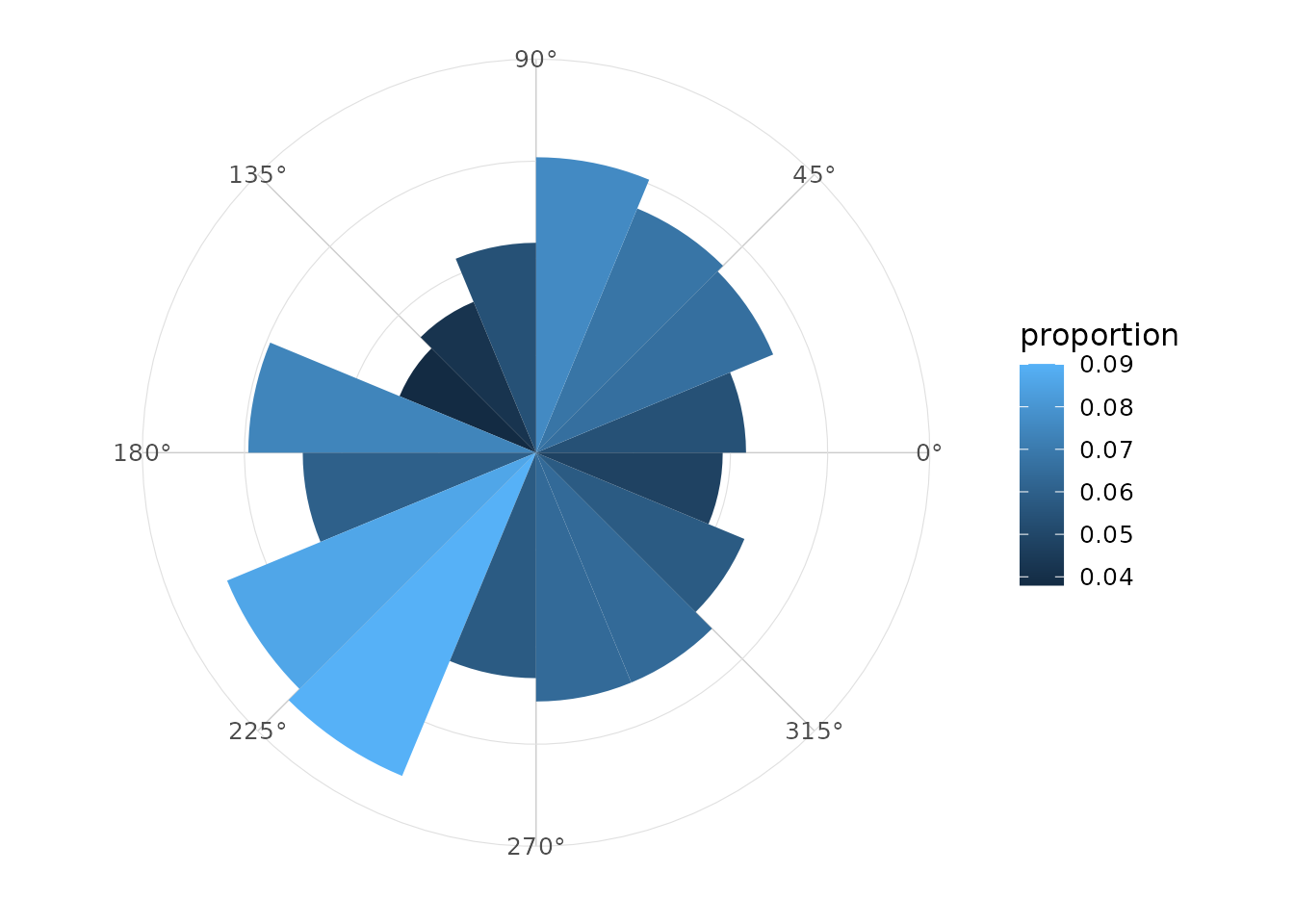
Groups and facets
Because the layers follow the ggplot2 grammar, standard
grouping, colouring and faceting workflows work naturally.
ggplot(wind_directions, aes(x = direction, fill = season)) +
  geom_rose(bins = 16, alpha = 0.75) +
  facet_wrap(~ season) +
  scale_x_circular_degrees() +
  coord_circular() +
  theme_circular()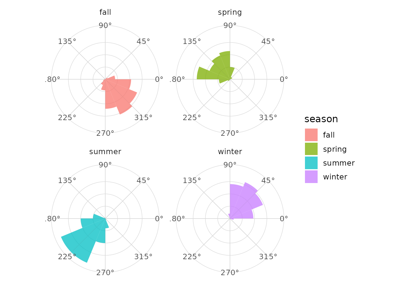
Circular density
geom_circular_density() estimates a smooth density on
the circle using a von Mises kernel. The estimate wraps around the
origin.
ggplot(wind_directions, aes(x = direction)) +
  geom_rose(aes(y = after_stat(density)), bins = 24, alpha = 0.35) +
  geom_circular_density(linewidth = 1) +
  scale_x_circular_degrees() +
  coord_circular() +
  theme_circular()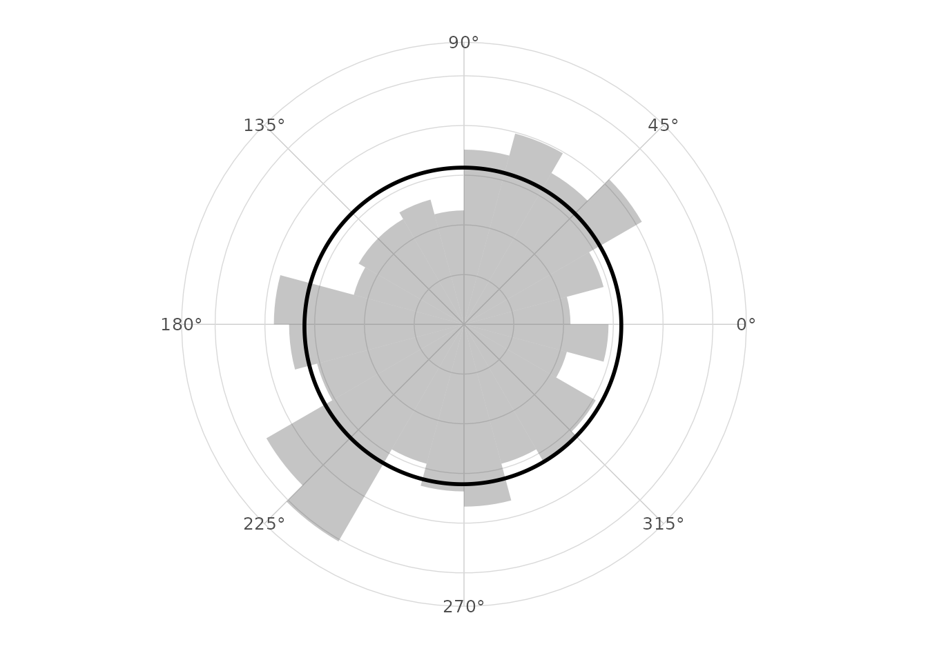
The bandwidth can be adjusted. Smaller values show more local variation.
ggplot(wind_directions, aes(x = direction)) +
  geom_circular_density(bw = 0.25, linewidth = 1) +
  geom_circular_density(bw = 0.75, linetype = 2) +
  scale_x_circular_degrees() +
  coord_circular() +
  theme_circular()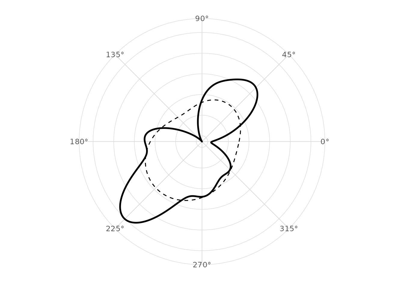
Mean direction and resultant length
The mean resultant length Rbar measures concentration.
Values close to one indicate strong concentration; values close to zero
indicate weak or cancelling directionality.
wind_directions |>
  group_by(season) |>
  circular_summary(direction)
#> # A tibble: 4 × 8
#>   season     n  mean     R  Rbar variance    sd kappa
#>   <chr>  <int> <dbl> <dbl> <dbl>    <dbl> <dbl> <dbl>
#> 1 fall     131 5.42  106.  0.811   0.189  0.647  3.00
#> 2 spring   115 2.36   92.3 0.802   0.198  0.664  2.89
#> 3 summer   138 3.90  120.  0.870   0.130  0.528  4.15
#> 4 winter   116 0.842 105.  0.904   0.0956 0.448  5.52
ggplot(wind_directions, aes(x = direction, colour = season)) +
  geom_circular_density(linewidth = 1) +
  geom_mean_direction(length = "resultant") +
  scale_x_circular_degrees() +
  coord_circular() +
  theme_circular()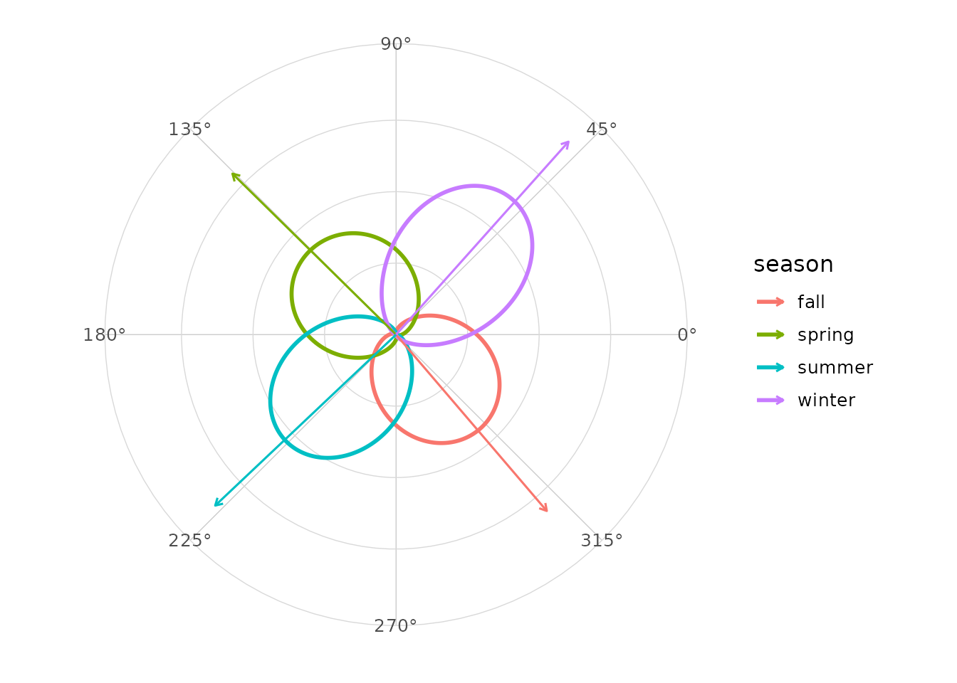
Uncertainty and circular tests
circular_mean_ci() computes large-sample or bootstrap
intervals for the mean direction. rayleigh_test() provides
a basic test against circular uniformity.
circular_mean_ci(wind_directions$direction, method = "large_sample")
#> # A tibble: 1 × 7
#>    mean lower upper level method           n   Rbar
#>   <dbl> <dbl> <dbl> <dbl> <chr>        <int>  <dbl>
#> 1  4.10  3.72  4.49  0.95 large_sample   500 0.0494
rayleigh_test(wind_directions$direction)
#>
#>  Rayleigh test of circular uniformity
#>
#> data:  c(3.61399414214871, 0.516403808686312, 3.18127143608671, 2.81398312066174, 3.48203785207672, 0.56424680709192, 0.629856683201911, 5.13158541730147, 0.857734675514404, 5.52884932182807, 6.14565025509431, 3.39186111855533, 5.68072279739308, 4.61418407964105, 4.74543931715619, 0.561767051885953, 3.93703683208835, 4.27621516412755, 0.88537547466561, 3.38244973375004, 4.54086340127989, 0.0252624877997549, 4.27062854516948, 3.97637694706441, 5.85083657554049, 5.87445936548537, 1.58836065931894, 3.77285531449948, 2.84978104987197, 3.65012027729075, 5.46563648989713, 4.10415613798566, 3.75388329273006, 3.98584710606474, 2.82144437086184, 1.50629832290545, 2.18486780537149, 1.55751051364113, 0.0276964845286848, 1.50071871494719, 5.4254641199483, 0.543084919785049, 3.16092065452067, 5.19124427895539, 6.19464201355272, 1.95365834413386, 1.75825901233488, 1.52372125275916, 1.30632888111883, 0.592208207194502, 2.48457594188947, 4.31585345061938, 3.2081127490451, 0.491798377205358, 2.10165361682883, 5.06620154208669, 0.663659415378715, 3.8895585724636, 3.91314585258669, 1.06943034646083, 3.70329020667088, 2.88997331413771, 1.25949333727748, 1.10349295627909, 5.48850298910456, 1.47392385975173, 1.53744771382702, 3.27633450940558, 6.02390363373308, 6.04815804577962, 2.26952313373199, 2.90608819205143, 3.86241193458018, 5.67412084741953, 3.26452859880416, 6.15350006888704, 5.48688255166703, 6.20791616467307, 3.68384365075044, 0.171424413263971, 1.22289990351848, 0.753079742018805, 5.13935788342828, 2.45542670127482, 0.745611903805254, 2.90938404806413, 2.74702586427139, 2.9514284893538, 2.27968831808027, 4.21823280781812, 4.30722391611882, 4.35748350312151, 5.65527822664119, 2.58867423785994, 3.13349236913869, 4.92601382435363, 1.3803664201544, 3.98074646585331, 0.241589583703272, 2.89416586974954, 4.78777809195007, 4.83810271328066, 1.79223368965479, 0.511613556058242, 4.3573339243357, 5.28646241936886, 0.527295585374115, 1.18807009034664, 5.83711134904222, 1.36989616319516, 2.87273782201903, 0.915014496611803, 2.32383561388706, 1.07966269956572, 4.01434607511189, 0.78462043869988, 5.46885293945382, 2.0118951346537, 5.55594286546511, 5.12698629884893, 1.19399119318522, 4.6409638519865, 0.372762827035868, 1.45477015543137, 6.1665437109926, 1.28558438743651, 3.84557068529067, 1.52635330490985, 3.07239368846469, 6.11836229228667, 5.51099187302794, 3.93918610415792, 3.56348178691564, 4.49677867159495, 3.85603721315972, 5.27373647197434, 4.48989903834052, 3.95919733894795, 3.6631658843697, 3.91174484376691, 2.23336435474006, 4.66503636345594, 5.69533325146029, 4.18078449624687, 1.17748434276607, 4.51542532015402, 1.38092818189996, 3.95863852463007, 4.86465650655373, 0.600031048441578, 5.64903433508069, 1.49945938128569, 1.13458378165887, 0.318720239109591, 0.937741030581609, 5.12272810621474, 2.69642747561964, 4.01835946823438, 0.821530057207844, 1.95574045975733, 0.952019577721132, 0.128785533480376, 1.93701079091507, 0.622326941415605, 3.81490338273784, 5.83318150760357, 4.80788354300373, 0.883680527329103, 2.03227696333366, 4.97480147885834, 2.53652203973757, 1.74609782105209, 5.31644410247321, 0.903501240888298, 1.40581408618352, 3.21798275606962, 3.4557590373251, 2.95845594631303, 1.24035058000518, 3.87818094178941, 4.06566783092223, 0.343587710646396, 1.64113506597964, 0.678143008925494, 3.10340916394715, 2.5234856281277, 4.076998724402, 0.227939389240854, 3.75293327615498, 0.745681375843156, 1.79773893567552, 4.64801929729362, 1.94577117034086, 2.5558571758186, 2.39320922469584, 4.93891730713478, 2.32486289997962, 1.63037333578965, 3.31520453696742, 5.30841845365601, 0.372030516182691, 2.78085103499691, 2.40916313762562, 2.76513836870851, 1.59553887068255, 3.92070775491521, 5.05790011995272, 2.35287611790499, 2.96528228895961, 4.32666169122151, 5.9072978350119, 3.83027765097782, 3.2164940873178, 5.70351195300256, 0.93247661803657, 5.15238639384105, 0.663953990503612, 5.66157231365886, 3.26171462649326, 1.45713601377082, 3.2983967872763, 1.95136053171296, 3.23351222754238, 4.78975722517733, 4.78186452379316, 3.695640374107, 4.8271958451668, 3.46123341534021, 5.57630440902539, 4.26989964224631, 0.350949155615401, 4.85043816877712, 1.43186037992258, 2.9749726389762, 5.84270909645015, 1.05597071241368, 5.45235967630183, 3.84902337434668, 2.17245168749446, 3.04717565556487, 5.84461210176993, 5.36426807769498, 6.09912805998087, 4.96680757207252, 4.05948061120776, 2.07519546021824, 2.84033536028553, 0.168823611299175, 1.70977104893379, 5.92098890272642, 3.26949882414043, 5.23428948002588, 1.69190192004778, 6.19346211529975, 4.49696023320816, 6.19446684610556, 3.7893701417916, 3.49909055641389, 5.40819799265068, 1.8846391290683, 1.21393910596394, 1.21552400584744, 3.6349745442456, 2.4634378399828, 1.95306022103064, 0.676993988570905, 3.93214167937047, 1.54946198744965, 4.36385094219077, 4.20260744900989, 0.82460022269939, 1.96563404453465, 5.47075647306217, 3.49105040587683, 3.32335522684759, 3.33345535109043, 5.84242928774451, 4.31021463398591, 0.830616800713155, 1.87429063250033, 4.63676047700973, 2.98274202524661, 5.32117631336934, 1.87580316931015, 4.14713947391929, 2.90022394794143, 6.02877873150384, 0.877728151162343, 0.766619044785883, 2.5228198449887, 1.18336686064368, 5.32978254102456, 0.480816221958569, 5.26714356331552, 4.43017298701401, 2.97367368861929, 0.741214166998673, 4.01559877502578, 0.305708772610524, 5.35578150769504, 5.67224213603809, 4.72340182475188, 5.10106676375622, 4.93432516183874, 3.54912615605738, 2.467008898568, 0.383693716213354, 4.1778110374832, 5.93580811375246, 2.22148314590711, 0.695143195391176, 2.56660094585538, 3.86451460546857, 4.75595722432728, 1.85086408782989, 2.85188077385315, 1.13650012641987, 1.85183397114663, 0.760046058469871, 4.66854906429729, 4.59375721951795, 5.97713848300698, 4.86285468485826, 2.71991476947419, 2.30715292875096, 0.877103345327341, 2.53242534640893, 4.61919504110127, 1.59021218025985, 2.01634243854563, 6.03532149675354, 3.52272992491007, 6.20511867529189, 2.94036438670711, 4.28094051000119, 6.08817754236178, 4.28050227060493, 3.94257340390048, 2.27807075458384, 0.37966828266774, 1.07007046003566, 3.6314960185085, 3.85761184272218, 0.290280604702401, 5.77985344386501, 5.83270710164554, 1.0174845770154, 2.89615963673962, 1.58107936514707, 5.91740372236149, 0.970114871729027, 1.42482016242241, 6.16857082735071, 2.76323109090468, 1.50286652193992, 2.10460490221135, 5.24362452608994, 3.67674993950874, 4.684245743071, 5.06986407882866, 4.19961987159562, 4.06181456709559, 3.71015031090074, 0.568004519325911, 5.02362397605336, 4.06902374222269, 4.00670250402605, 3.99406586291155, 3.02690407702263, 0.24204898447192, 3.67884707982449, 4.17390245121511, 1.0501552383401, 5.48554177000912, 3.2534035574453, 0.607437218823521, 2.32387054099722, 4.68929088864066, 5.63270291232151, 1.06305238835461, 1.40510154106626, 1.33926684832572, 2.9193216111759, 1.36233590748847, 5.47739489161281, 3.65710105949873, 0.276645059413112, 0.176706690397123, 1.32381779895136, 3.13413908979964, 0.967610140820129, 3.19004724297362, 3.73572342516266, 0.698842921725046, 4.87416618466692, 5.15402319845046, 4.17140260230116, 5.00153849029061, 0.497819145365931, 4.20328951404635, 0.702392839987015, 3.829295278135, 4.73868633902796, 2.99753719488559, 4.05278142217793, 4.67147517252104, 5.06141329630149, 5.54698117956277, 4.11173633921752, 0.165202227483394, 3.91069891339029, 0.383561820290968, 1.55022261592284, 3.25518382541973, 3.84110621092413, 4.56659839277621, 1.08653834341982, 3.04694149757914, 4.48987968990351, 5.11734368389185, 5.66475271719934, 4.17889337704655, 2.85817235346097, 2.6159630514743, 3.03108419307564, 5.54107102563832, 3.53607034711238, 6.26809787788282, 2.31698401678689, 3.74576011697637, 0.864108209209264, 1.5802118303633, 3.6517313682625, 3.36357147943932, 4.58533773954467, 3.19103194878316, 4.03384706710371, 4.76106093475281, 4.81901276141423, 1.23977284481888, 4.12784986364102, 3.56797141334475, 0.896458792049424, 3.70970605097961, 3.54969636829351, 3.2062230604813, 2.77985955675029, 1.22432857910086, 4.93259138319717, 2.46775799862233, 3.0081898503984, 4.46876212802286, 4.57781331054168, 0.552753637975135, 0.324650573480147, 0.728226014527112, 3.93153251949303, 1.21838451558546, 5.20699823430224, 6.24801251078914, 0.239056878808596, 1.02192634247736, 1.85186911144518, 5.62985543179424, 0.816738462684404, 0.8208128687534, 4.79467712783871, 1.22335103227416, 6.15681766244913, 2.18445569446985, 4.02130822642411, 2.57709436969584, 5.71567719459435, 5.55723921768227, 4.36715762912422, 0.00707276489959519, 3.40550301804636, 4.02396304780405, 0.146235683957278, 2.89089615037712, 5.14749594931166, 0.416423364443049, 1.6892383377323, 5.45251947827975, 3.68341682083734, 5.65190756066476, 3.6106115015918, 1.62664317760994, 0.679671124258451, 1.25048140461135, 0.325155400571825, 3.29802486918288, 4.76912826669582, 2.8726142700713, 4.60731046578359, 4.43142878290656, 0.16599519498687, 4.97133206466733, 0.873701166879113, 0.826052507566032)
#> z = 1.2207, n = 500, p-value = 0.2952
#> alternative hypothesis: the distribution is unimodal and non-uniform
ggplot(wind_directions, aes(x = direction)) +
  geom_rose(bins = 16, alpha = 0.8) +
  stat_circular_test(test = "rayleigh", y = 1.1, size = 3) +
  scale_x_circular_degrees() +
  coord_circular() +
  theme_circular()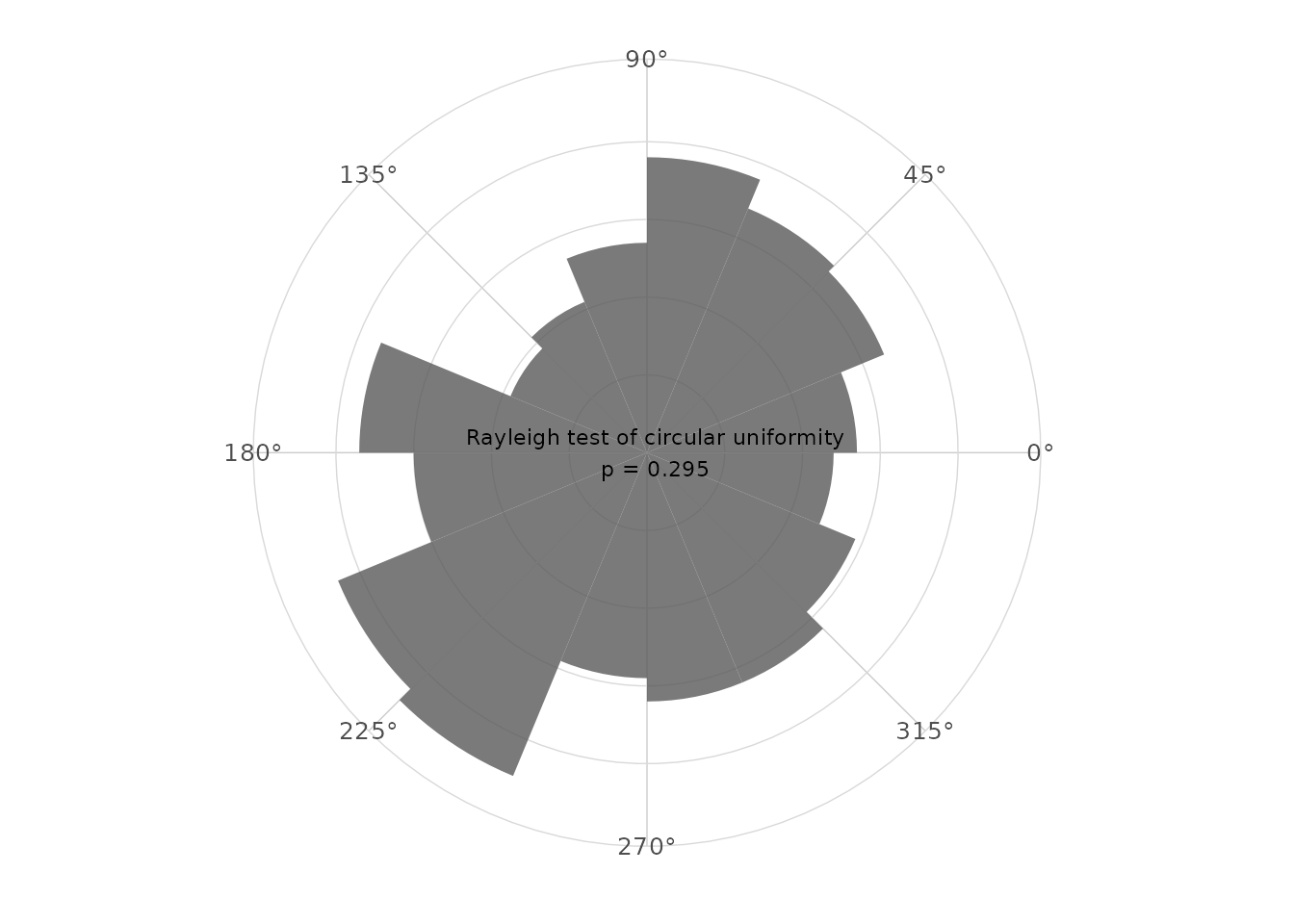
Compass display
For bearing-like data, compass labels and geographic orientation are usually easier to read.
ggplot(wind_directions, aes(x = direction)) +
  geom_rose(bins = 16, aes(fill = after_stat(count))) +
  geom_mean_direction() +
  scale_x_circular_compass() +
  coord_circular(zero = "north", direction = "clockwise") +
  theme_compass()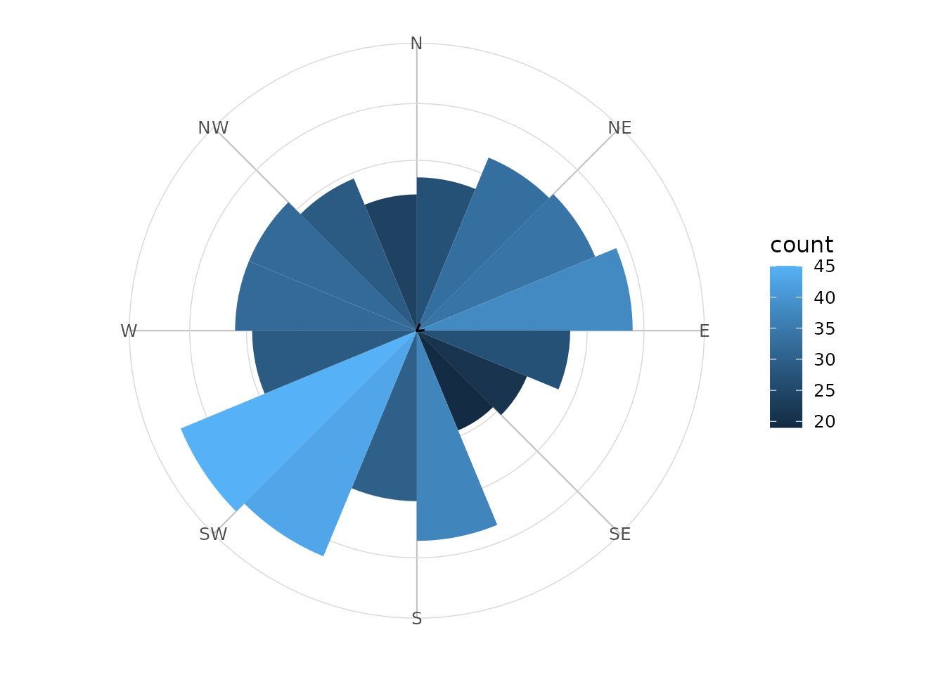
Axial data
Set axial = TRUE when orientations are modulo
pi.
axial_orientations |>
  group_by(group) |>
  circular_summary(orientation, axial = TRUE)
#> # A tibble: 3 × 8
#>   group     n  mean     R  Rbar variance    sd kappa
#>   <chr> <int> <dbl> <dbl> <dbl>    <dbl> <dbl> <dbl>
#> 1 A       107 0.370 100.0 0.935   0.0655 0.368  7.91
#> 2 B       108 1.02  100.  0.928   0.0718 0.386  7.24
#> 3 C        85 1.25   77.7 0.915   0.0855 0.423  6.13
ggplot(axial_orientations, aes(x = orientation, fill = group)) +
  geom_rose(bins = 18, axial = TRUE, alpha = 0.7) +
  geom_mean_direction(axial = TRUE) +
  scale_x_circular_degrees(limits = c(0, pi)) +
  coord_circular() +
  theme_circular()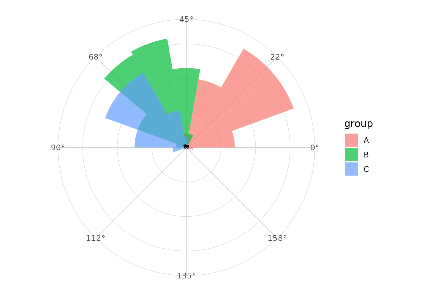
Movement data
Movement tracks naturally produce step lengths, bearings and turn angles.
animal_steps |>
  group_by(state) |>
  summarise(
    mean_step = mean(step_length, na.rm = TRUE),
    median_step = median(step_length, na.rm = TRUE),
    .groups = "drop"
  )
#> # A tibble: 3 × 3
#>   state       mean_step median_step
#>   <chr>           <dbl>       <dbl>
#> 1 directed        3.30        3.23
#> 2 encamped        0.471       0.382
#> 3 exploratory     1.35        1.20
ggplot(animal_steps, aes(x = x, y = y, group = id, colour = id)) +
  geom_path(alpha = 0.7) +
  coord_equal() +
  theme_minimal()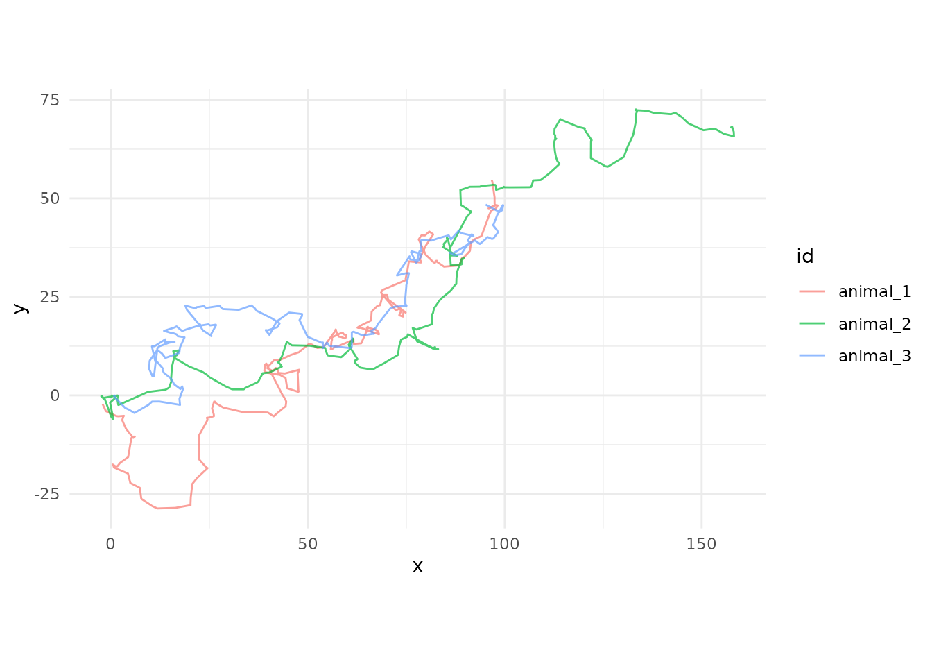
plot_state_angles(animal_steps, angle = turn_angle, state = state, type = "rose")
#> Warning: Removed 280 rows containing non-finite outside the scale range
#> (`stat_rose()`).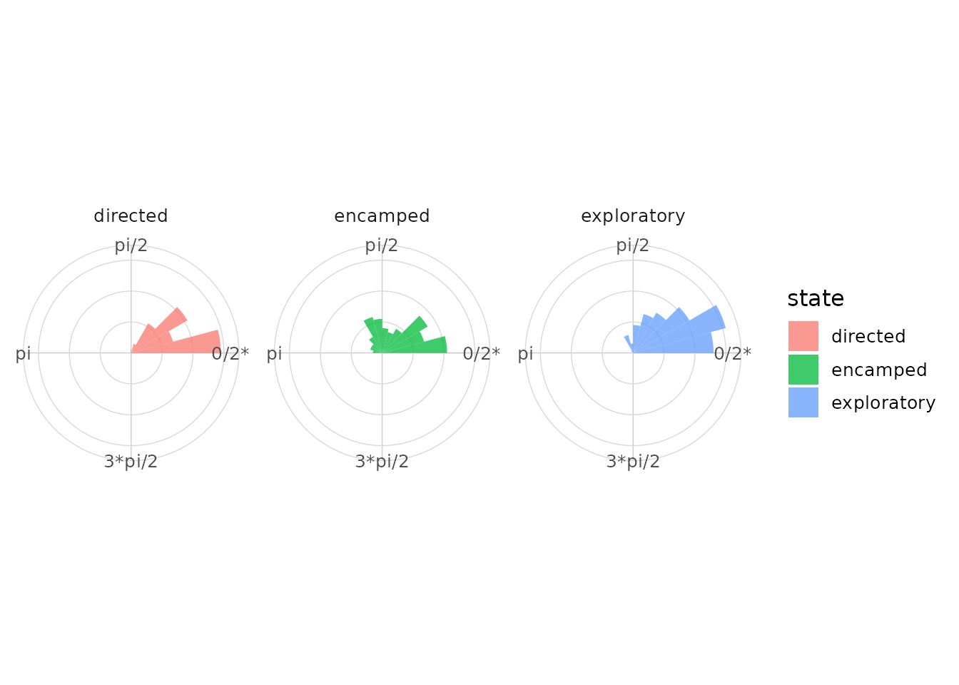
plot_state_angles(animal_steps, angle = turn_angle, state = state, type = "density")
#> Warning: Removed 280 rows containing non-finite outside the scale range
#> (`stat_circular_density()`).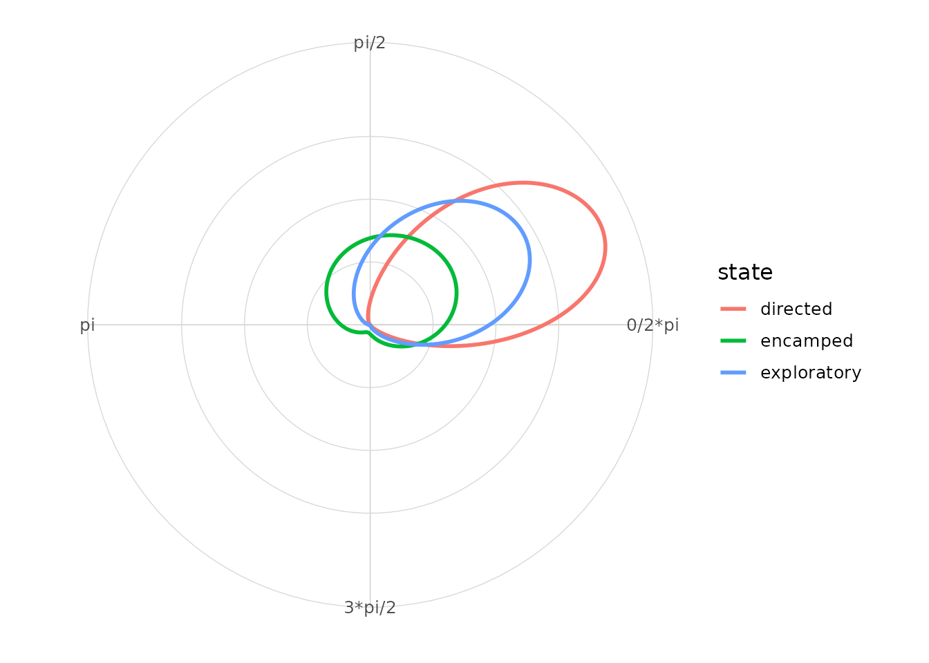
Mixtures of von Mises distributions
Mixtures provide a descriptive way to represent multimodal circular
distributions. The EM fit can depend on initialization, so use
seed, nstart and
glance_circular() when reproducibility or convergence
matters.
fit_mix <- fit_vonmises_mixture(
  wind_directions$direction,
  k = 2,
  nstart = 3,
  seed = 2026,
  max_iter = 200
)
#> Warning: `fit_vonmises_mixture()` did not converge within `max_iter`
#> iterations.

tidy_circular(fit_mix)
#> # A tibble: 2 × 4
#>   component proportion    mu kappa
#>       <int>      <dbl> <dbl> <dbl>
#> 1         1      0.321 0.903 1.49
#> 2         2      0.679 4.06  0.755
glance_circular(fit_mix)
#> # A tibble: 1 × 12
#>       n components logLik   AIC   BIC iterations converged nstart start_id
#>   <int>      <int>  <dbl> <dbl> <dbl>      <int> <lgl>      <int>    <int>
#> 1   500          2  -912. 1833. 1854.        200 FALSE          3        1
#> # ℹ 3 more variables: empty_components <int>, kappa_max <dbl>, axial <lgl>
ggplot(wind_directions, aes(x = direction)) +
  geom_rose(aes(y = after_stat(density)), bins = 24, alpha = 0.35) +
  stat_vonmises_mixture(fit = fit_mix, linewidth = 1) +
  scale_x_circular_degrees() +
  coord_circular() +
  theme_circular()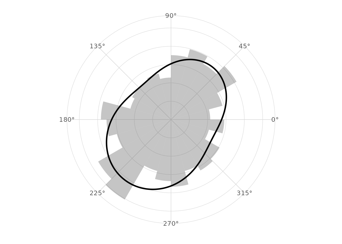
Angular model diagnostics
ggcircular provides basic methods for angular model
summaries and residual diagnostics. The example below uses a small mock
object with the same observed and fitted angle fields expected from
supported angular model classes.
fit <- structure(
  list(
    y = wind_directions$direction[1:50],
    mui = normalize_angle(wind_directions$direction[1:50] + rnorm(50, 0, 0.15)),
    term_labels = c("intercept", "speed")
  ),
  class = "angular"
)

tidy_circular(fit)
#> # A tibble: 2 × 2
#>   term      estimate
#>   <chr>        <dbl>
#> 1 intercept        0
#> 2 speed            0
glance_circular(fit)
#> # A tibble: 1 × 7
#>   model_class  nobs  npar logLik   AIC   BIC kappa
#>   <chr>       <int> <int>  <dbl> <dbl> <dbl> <dbl>
#> 1 angular        50     0     NA    NA    NA    NA
circular_model_diagnostics(fit)
#> # A tibble: 1 × 6
#>   model_class     n residual_mean residual_Rbar residual_variance
#>   <chr>       <int>         <dbl>         <dbl>             <dbl>
#> 1 angular        50        0.0143         0.987            0.0126
#> # ℹ 1 more variable: max_abs_residual <dbl>
autoplot(fit, type = "residuals_density")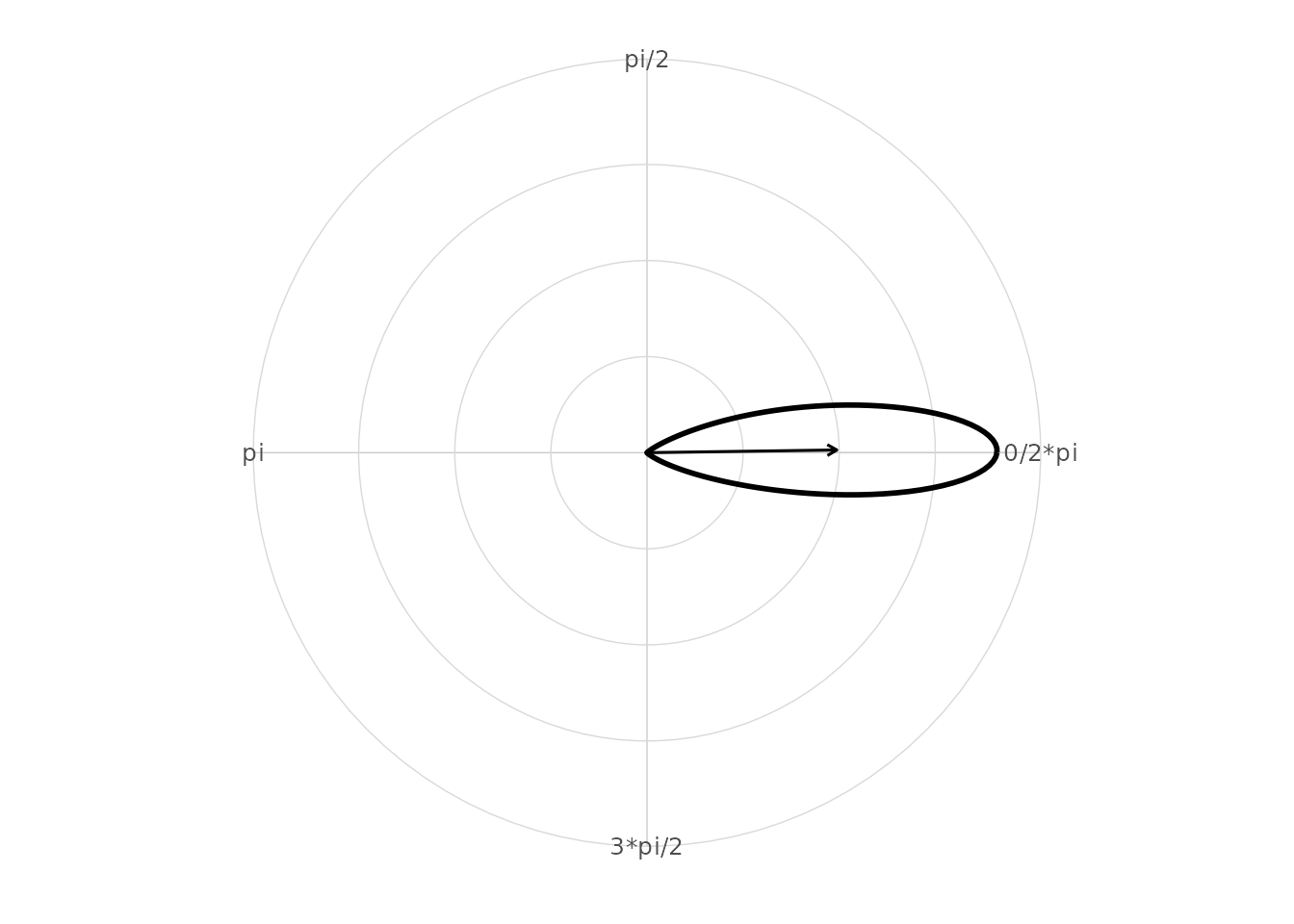
Circular posterior draws
When the optional posterior package is installed,
circular posterior draws can be converted to a long format and
summarized with circular statistics.
if (requireNamespace("posterior", quietly = TRUE)) {
  set.seed(1)
  draws <- posterior::draws_df(
    theta = rnorm(400, mean = pi / 3, sd = 0.25),
    phi = rnorm(400, mean = pi, sd = 0.35)
  )

  circular_draws <- as_circular_draws(draws, variables = c("theta", "phi"))
  summarise_circular_draws(circular_draws)
}
#> # A tibble: 2 × 7
#>   .variable     n  mean  Rbar lower upper level
#>   <chr>     <int> <dbl> <dbl> <dbl> <dbl> <dbl>
#> 1 phi         400  3.12 0.931 2.37   3.83  0.95
#> 2 theta       400  1.06 0.971 0.567  1.52  0.95
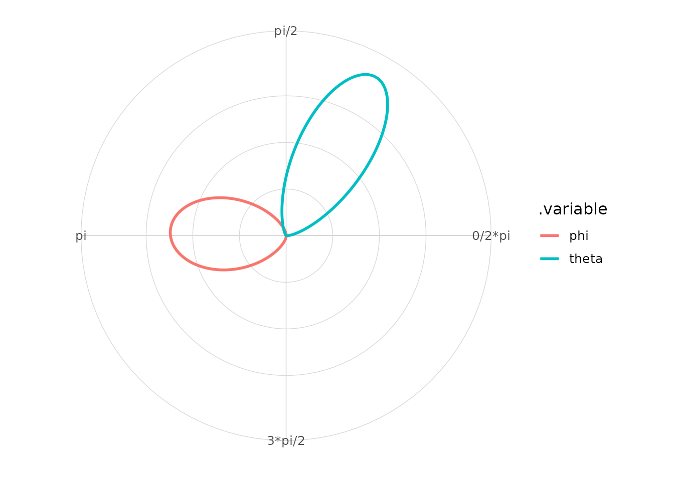
if (requireNamespace("posterior", quietly = TRUE)) {
  autoplot_circular_draws(circular_draws)
}
Experimental features
The optional model integrations are experimental. They are intended
to make diagnostics easier for workflows built with
CircularRegression, momentuHMM and
posterior, while keeping those packages in
Suggests. The functions give explicit errors when an
optional package is required but not installed.
Statistical limitations
Circular graphics are descriptive and should be read with the data-generating context in mind.
- A rose diagram can change visually with the number of bins.
- A circular mean is unstable when
Rbaris close to zero. - Directional and axial data require different summaries.
- Compass bearings and mathematical angles use different zero directions.
- Multimodal data should not be summarized only by one mean direction.
- The automatic circular density bandwidth is a heuristic.
-
estimate_kappa()is a descriptive approximation, not a full uncertainty analysis. - Rayleigh and Watson-Williams tests have classical assumptions that should be checked before confirmatory use.