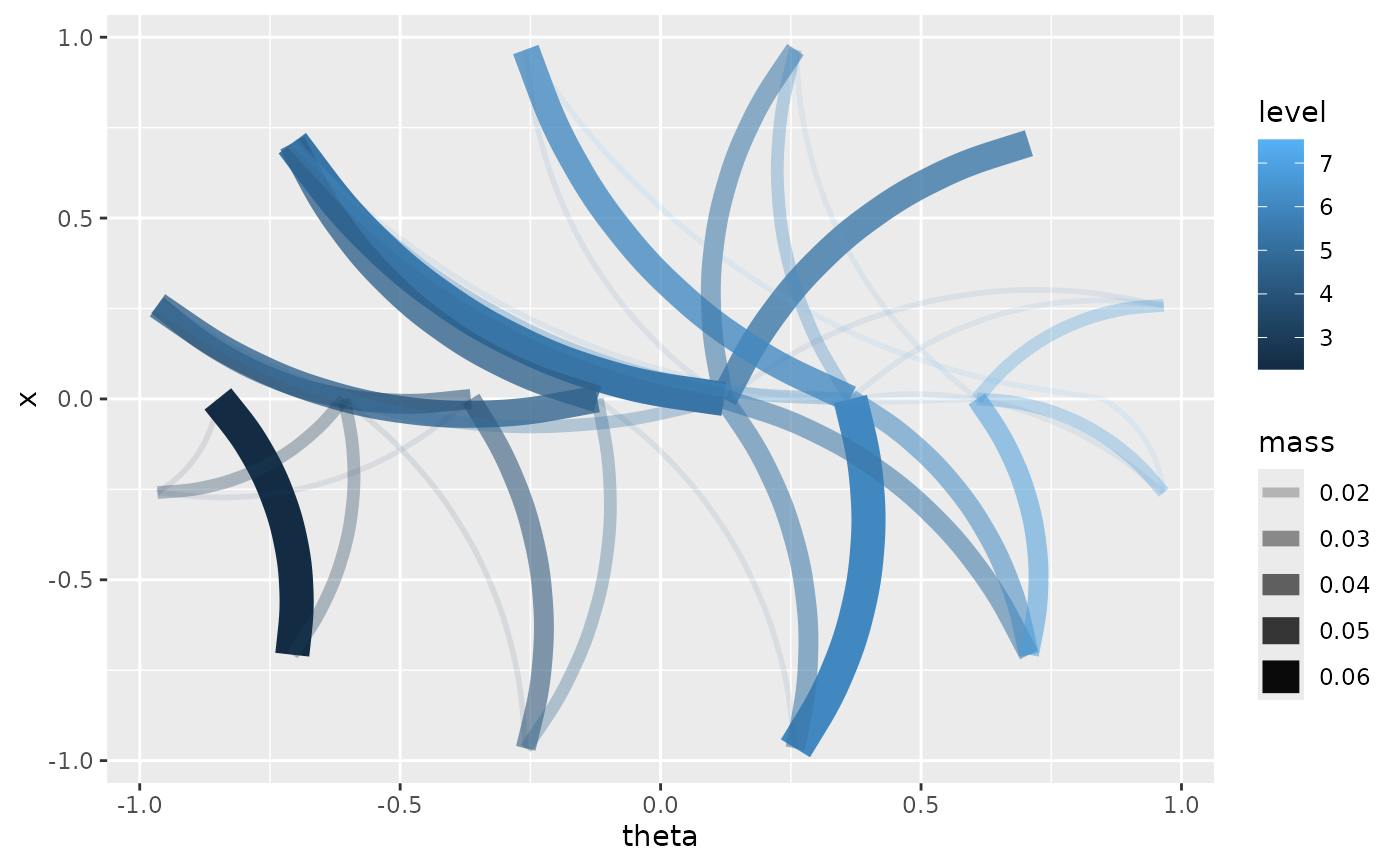
Add a phase loom layer — geom_phase_loom • ggcircular

Adds mass-flow curves for circular-linear data. Use this layer with ggplot2::ggplot(data, ggplot2::aes(x = theta, y = response)).

Usage

geom_phase_loom(
  mapping = NULL,
  data = NULL,
  position = "identity",
  n_sectors = 48,
  n_x_bins = 24,
  min_mass = 0.002,
  max_flows = 180,
  mass_type = c("joint", "conditional"),
  curvature = 0.24,
  ...,
  show.legend = NA,
  inherit.aes = TRUE
)

Arguments

mapping, data, position, show.legend, inherit.aes: Standard ggplot2 layer arguments.
n_sectors: Number of angular sectors.
n_x_bins: Number of bins for the linear response.
min_mass: Minimum mass to draw.
max_flows: Maximum number of flows to draw. Use NULL to draw all.
mass_type: Either "joint" or "conditional".
curvature: Curvature passed to ggplot2::geom_curve().
...: Additional arguments passed to the geom.

Value

A ggplot2 layer.

See also

Other cylindrical dependence layers: stat_circular_topography(), stat_statistical_orbit(), stat_statistical_orbit_ribbon()

Examples

dat <- simulate_cylindrical(n = 80, seed = 1)
ggplot2::ggplot(dat, ggplot2::aes(x = theta, y = x)) +
  geom_phase_loom(n_sectors = 12, n_x_bins = 8, min_mass = 0)