Visualizing Circular and Directional Data with ggcircular

Abstract

This demonstration presents a reproducible workflow for simulated animal movement data. The aim is to show how rose diagrams, circular density estimates and mean directions can be combined in a ggplot2 grammar.

Introduction

Directional variables occur in wind, movement, orientation and time-of-day data. Their periodic nature requires summaries and graphics that respect the circle.

Circular data and specialized graphics

Circular graphics should keep the endpoints of the angular scale adjacent. They should also distinguish directionality, concentration and uncertainty.

The grammar of ggcircular

library(ggplot2)
library(dplyr)
#> 
#> Attaching package: 'dplyr'
#> The following objects are masked from 'package:stats':
#> 
#>     filter, lag
#> The following objects are masked from 'package:base':
#> 
#>     intersect, setdiff, setequal, union
library(ggcircular)

Simulated trajectories

ggplot(animal_steps, aes(x = x, y = y, group = id, colour = id)) +
  geom_path(alpha = 0.7) +
  coord_equal() +
  theme_minimal()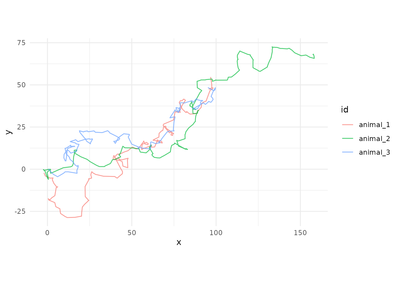

Directional features

movement_summary <- animal_steps |>
  group_by(state) |>
  summarise(
    mean_step = mean(step_length, na.rm = TRUE),
    median_step = median(step_length, na.rm = TRUE),
    .groups = "drop"
  )

movement_summary
#> # A tibble: 3 × 3
#>   state       mean_step median_step
#>   <chr>           <dbl>       <dbl>
#> 1 directed        3.30        3.23 
#> 2 encamped        0.471       0.382
#> 3 exploratory     1.35        1.20

Bearings by state

ggplot(animal_steps, aes(x = bearing, fill = state)) +
  geom_rose(bins = 24, alpha = 0.7) +
  facet_wrap(~ state) +
  scale_x_circular_degrees() +
  coord_circular() +
  theme_circular()
#> Warning: Removed 3 rows containing non-finite outside the scale range
#> (`stat_rose()`).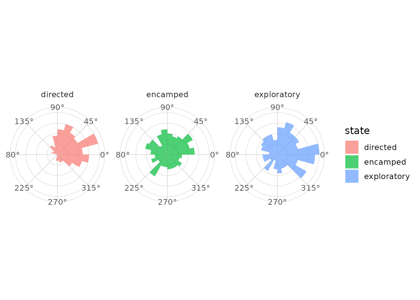

Turn angles by state

ggplot(animal_steps, aes(x = turn_angle, fill = state)) +
  geom_rose(bins = 24, alpha = 0.7) +
  geom_mean_direction() +
  facet_wrap(~ state) +
  scale_x_circular_radians() +
  coord_circular() +
  theme_circular()
#> Warning: Removed 280 rows containing non-finite outside the scale range
#> (`stat_rose()`).
#> Warning: Removed 280 rows containing non-finite outside the scale range
#> (`stat_mean_direction()`).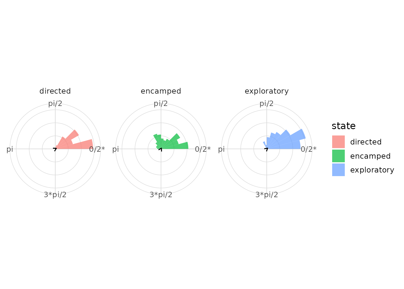

Mean directions and resultant length

animal_steps |>
  group_by(state) |>
  circular_summary(turn_angle)
#> # A tibble: 3 × 8
#>   state           n   mean     R  Rbar variance    sd kappa
#>   <chr>       <int>  <dbl> <dbl> <dbl>    <dbl> <dbl> <dbl>
#> 1 directed      153 0.0601 131.  0.856    0.144 0.558 3.78 
#> 2 encamped      207 0.203   57.6 0.278    0.722 1.60  0.579
#> 3 exploratory   234 0.0822 159.  0.679    0.321 0.880 1.88

Circular densities

ggplot(animal_steps, aes(x = turn_angle, colour = state)) +
  geom_circular_density(linewidth = 1) +
  scale_x_circular_radians() +
  coord_circular() +
  theme_circular()
#> Warning: Removed 280 rows containing non-finite outside the scale range
#> (`stat_circular_density()`).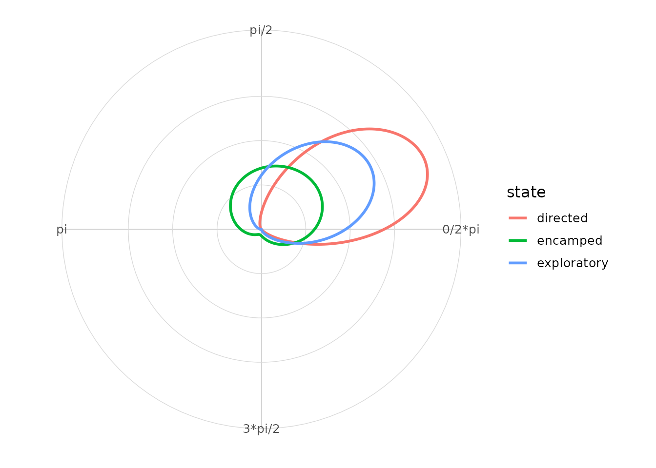

Interpretation

In the simulated data, directed movement has longer steps and more concentrated turn angles. Encamped movement has shorter steps and more diffuse turning. Exploratory movement is intermediate. These statements describe the simulated dataset and should not be generalized beyond it.

Discussion

The example shows how the same grammar can summarize raw angular observations, derived movement quantities and grouped comparisons.

Reproducibility

All data used here are included in the package as simulated datasets. The code chunks can be evaluated after installing ggcircular.