Circular-circular workflow

This vignette shows a basic circular-circular workflow. Both variables are angles, so the sample space is a torus.

library(ggplot2)
library(ggcircular)

dat <- simulate_tor_diagnostic(
  n = 260,
  scenario = "diagonal",
  seed = 2
)

The toroidal flow displays conditional binned mass between angular sectors. The toroidal topography estimates f(phi | theta). The conditional ridge extracts a dominant modal relation.

plot_toroidal_flow(dat$theta, dat$phi, n_sectors = 18)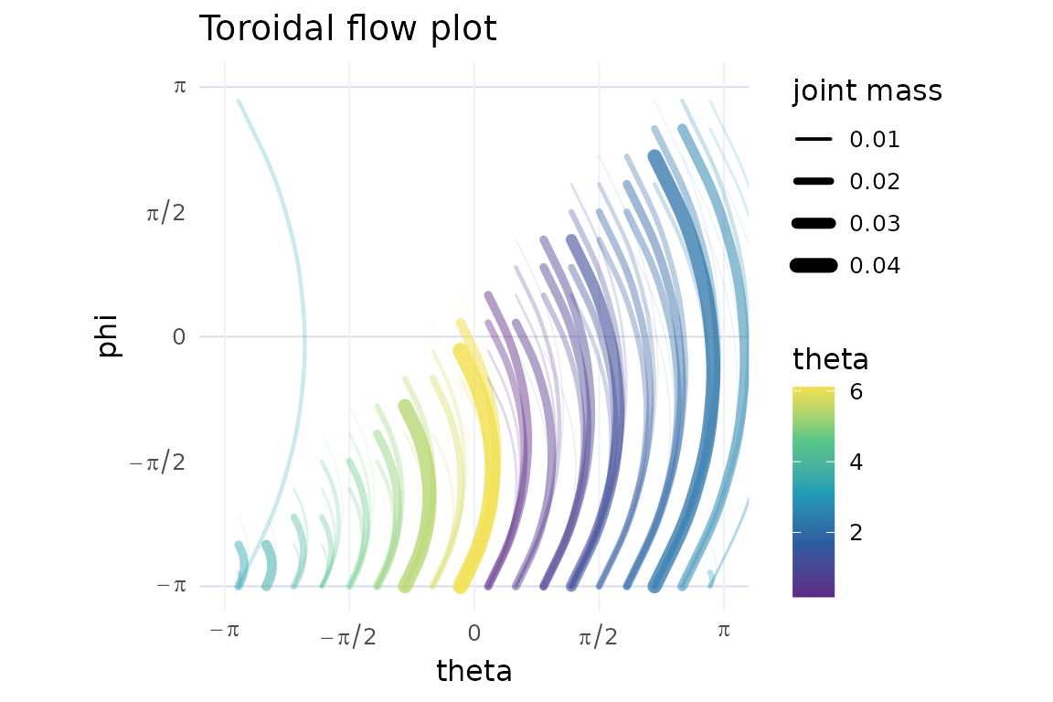

plot_toroidal_topography(dat$theta, dat$phi, n_theta = 50, n_phi = 50, conditional = TRUE)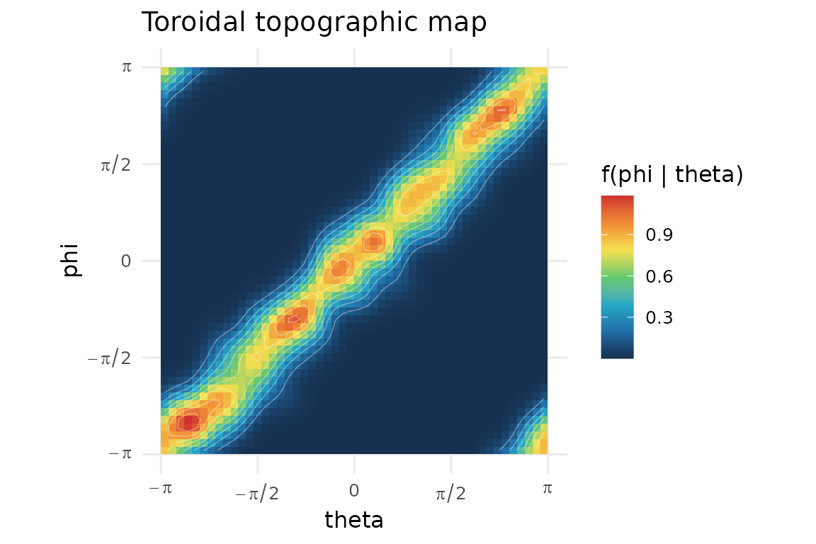

plot_toroidal_ridge(dat$theta, dat$phi, n_theta = 50, n_phi = 50)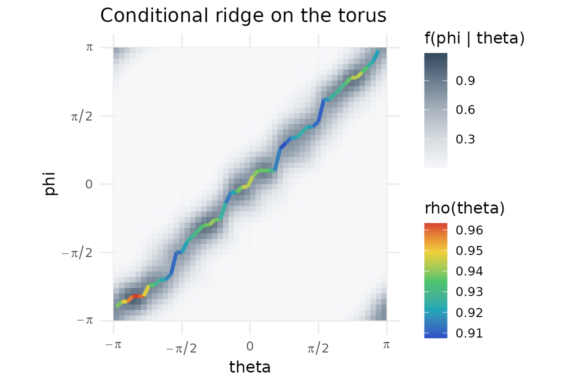

The ridge keeps the first exact grid maximum for reproducibility and backward compatibility. It also reports whether distinct local modes are nearly tied.

ridge <- toroidal_ridge_data(
  dat$theta,
  dat$phi,
  n_theta = 50,
  n_phi = 50,
  tie_tolerance = 0.01
)

table(ridge$ridge_ambiguous)
#> 
#> FALSE 
#>    50

The same displays can be built as ggplot2 layers.

ggplot(dat, aes(x = theta, y = phi)) +
  stat_toroidal_topography(n_theta = 50, n_phi = 50, conditional = TRUE) +
  stat_toroidal_ridge(n_theta = 50, n_phi = 50, linewidth = 1) +
  coord_equal()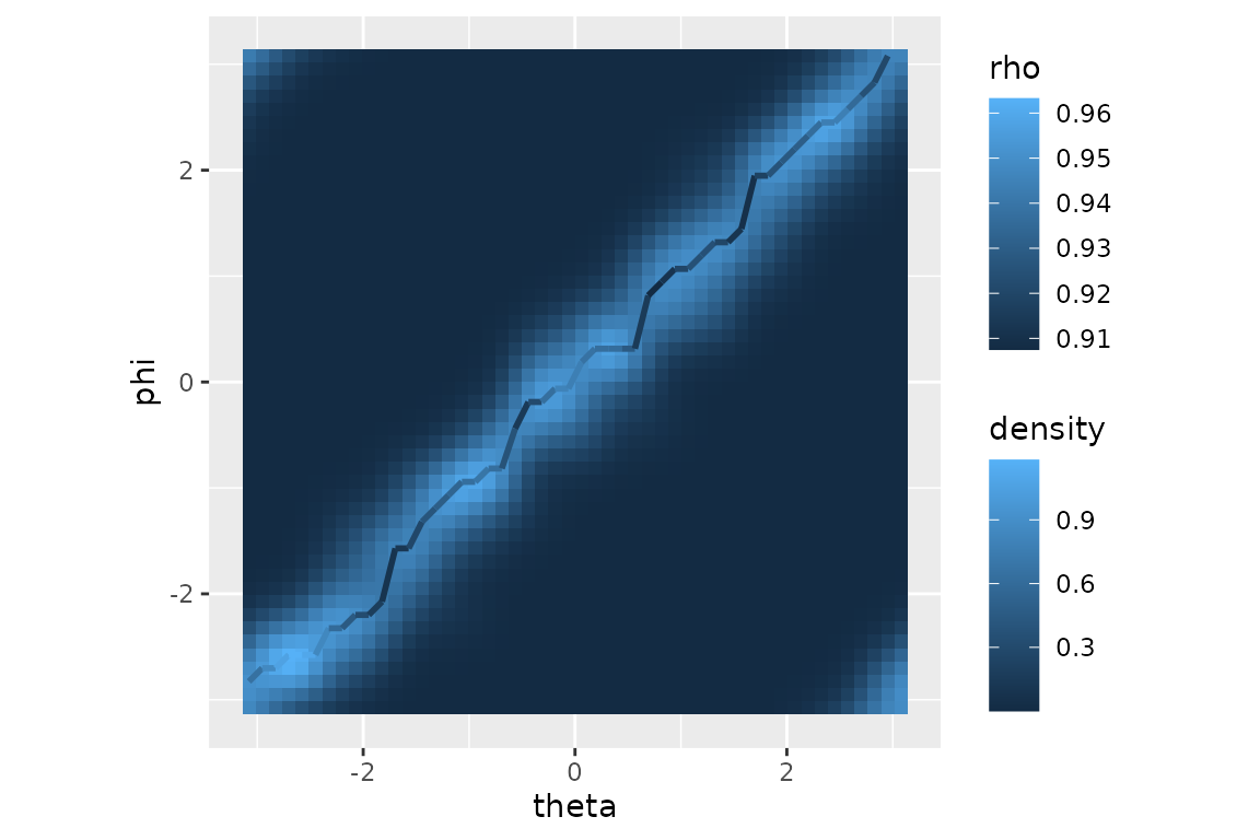

Exact ties select the first grid maximum. Near-ties are flagged when the ratio of the second-highest distinct local maximum to the highest local maximum is at least 1 - tie_tolerance. The selected curve is deterministic, but it is not stable under symmetric, multimodal or near-tied conditional densities. In those cases, use the topography as the primary display and do not interpret a single ridge in isolation.