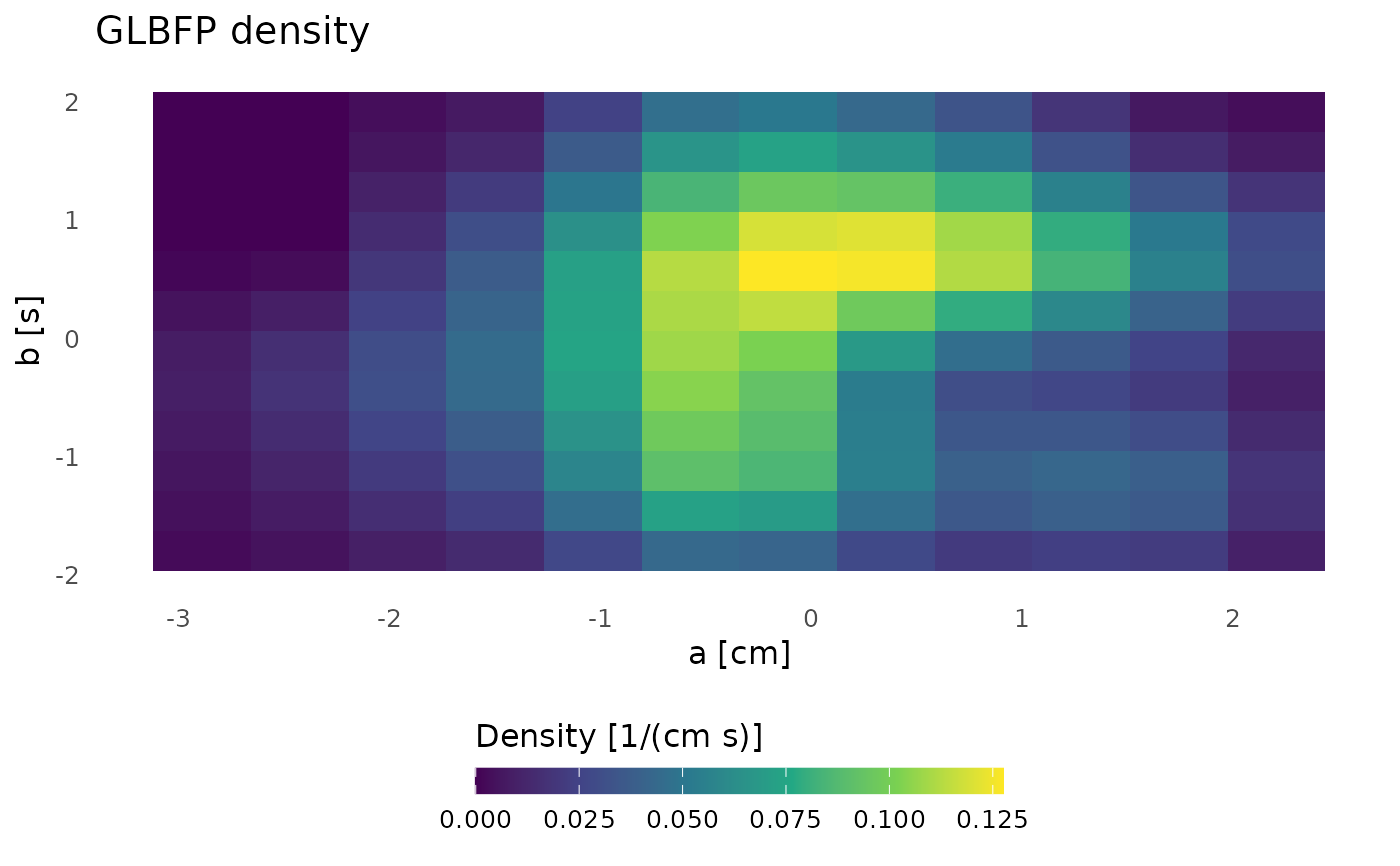
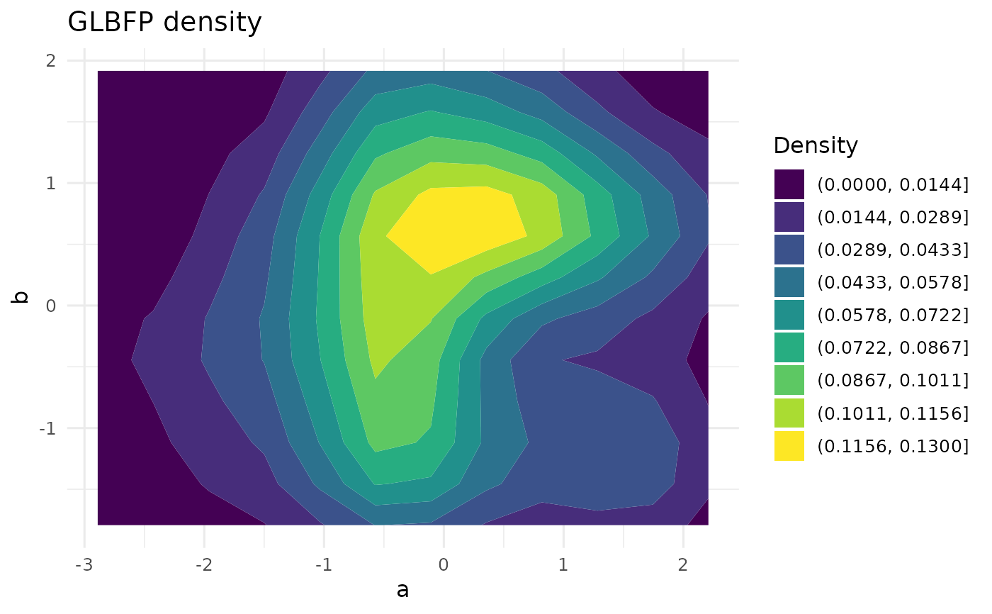
Visualize estimated densities in one to three observation dimensions

A surface for d=2 uses height for density. For d=3, all three spatial plot axes represent observation components; density is shown by slices or isosurfaces. Neither plot dimension refers to the index dimension N.

Usage

plot_density(
  x,
  type = NULL,
  labels = NULL,
  units = x$units,
  slice_dim = 3L,
  slices = NULL,
  isomin = NULL,
  isomax = NULL,
  surface_count = 3L,
  title = NULL
)

Arguments

x: A grid fit from GLBFP_estimate() or its ASH/LBFP counterparts.
type: "line", "heatmap", "contour", "surface", "slices", or "isosurface". Default depends on the observation dimension.
labels: Optional vector of observation axis labels (length d).
units: Optional vector of units (length d); defaults to field units. Density units are the reciprocal of their product, not the original units.
slice_dim: Observation dimension held fixed for slices (default 3).
slices: Values on that grid axis. Default uses up to three evenly spaced interior grid planes. A slice is a joint-density section, not a marginal or conditional density and is not renormalized.
isomin, isomax: Optional lower and upper isosurface density levels.
surface_count: Number of equally spaced isosurfaces (default 3).
title: Optional title.

Value

A ggplot for lines, heatmaps, contours and slices, or a plotly widget for surfaces/isosurfaces. Surfaces and volume plots require distinct complete Cartesian grids and at most 250,000 points. Unstructured 2D grids use points for legacy surface/contour requests; heatmaps reject them.

Examples

set.seed(20)
x <- cbind(a = rnorm(100), b = rnorm(100))
fit <- GLBFP_estimate(x, b = c(1, 1), grid_size = 12)
plot_density(fit, "heatmap", units = c("cm", "s"))

plot_density(fit, "contour")