Indexed fields: dimensions, grids and inference • GLBFP

Two different dimensions

The index dimension $N$ describes sites in $\mathbb{Z}^N$ . The observation dimension $d$ describes the random vector measured at each site. The density is a function on $\mathbb{R}^d$ , regardless of $N$ . Index coordinates are never silently used as observation components.

library(GLBFP)
set.seed(20261109)
field2 <- glbfp_field(array(rnorm(10 * 8), c(10, 8)), units = "standard unit")
field2
#> Indexed field: 80 observed sites; N = 2 ; d = 1 
#> Complete integer bounding box: TRUE 
#> Omitted sites: 0 ; dependence: unspecified
field3 <- glbfp_field(array(rnorm(5 * 4 * 3 * 2), c(5, 4, 3, 2)), value_dim = 4)
field3
#> Indexed field: 60 observed sites; N = 3 ; d = 2 
#> Complete integer bounding box: TRUE 
#> Omitted sites: 0 ; dependence: unspecified

Array entries are scalar observations by default. value_dim explicitly names the component axis for multivariate arrays. Alternatively, supply an $n \times d$ matrix of observations and a separate $n \times N$ matrix of integer sites.

sites <- as.matrix(expand.grid(i = 1:10, j = 1:8))
explicit <- glbfp_field(field2$values, indices = sites)
stopifnot(identical(field2$values, explicit$values))

Duplicate sites are rejected. Repeated observation values at different sites are allowed. Missing values cause an error unless na.action = "omit"; then the entire site is omitted and its coordinates recorded. Incomplete bounding boxes are accepted for descriptive marginal estimation without interpolation or imputation of missing sites. Their sampling design can change the interpretation of the empirical marginal distribution.

array_missing <- array(rnorm(80), c(10, 8))
array_missing[3, 4] <- NA_real_
incomplete <- glbfp_field(array_missing, na.action = "omit")
incomplete$complete
#> [1] FALSE
incomplete$omitted
#>      i1 i2
#> [1,]  3  4

Fixed grid and reusable counts

For bandwidth $b$ and integer parameter $m$ , the fine-cell width is $\delta=b/m$ . The anchor $a$ (specified by min_vals) defines half-open counting cells $[a+k\delta,\,a+(k+1)\delta)$ . Interpolation uses their centers. All unoccupied cells have zero counts on the full lattice. max_vals limits the display grid; it does not extrapolate, truncate or renormalize the density.

model <- prepare_glbfp(field2, b = .8, m = 2, min_vals = -5, max_vals = 5)
model
#> GLBFP prepared model: 80 observations, d = 1 
#> Occupied fine cells: 13 ; engine: cpp_direct
predict(model, matrix(c(-1, 0, 1), ncol = 1))
#> [1] 0.2578125 0.2890625 0.2304688
scores <- compute_Di(model)
summary(scores)
#> D_i score summary
#> Method: GLBFP 
#> Observations: 80 
#> Dimension: 1 
#> D_i quantiles:
#>         0%        25%        50%        75%       100% 
#> 0.02816594 0.03390363 0.03884178 0.06434040 0.32008753 
#> D_i mean: 0.06085209 
#> Missing D_i: 0 
#> Density range: 0.0364540786933973 to 0.304487593795238 
#> Median visited cells: 4 
#> Median prefix nodes: 4

The same preparation supports predictions and fixed-grid D_i scores. Native direct enumeration and prefix traversal have identical statistical targets. The faster engine depends on occupancy, stencil size and query count. The automatic threshold is a heuristic, not a universal optimum. Prefix traversal does not eliminate the combinatorial worst case.

What uncertainty means

The default returns no standard error or interval. Merely providing spatial indices does not justify independent sampling or an asymptotic normal law. For LBFP on a complete rectangular indexed field, an opt-in asymptotic method is available under the assumptions described below.

For independent observations, a fixed anchor, fixed bandwidths and fixed evaluation points, write the density estimate as the mean of observation weights $W_i(x)$ , including the factor $1/\prod_{j=1}^d b_j$ . The unbiased variance estimate is $\operatorname{var}\{W_i(x)\}/n$ . This identity does not need a small-bandwidth approximation. It does require IID sampling and fixed weights as functions of individual observations. A bandwidth selected from the same sample or an anchor equal to its minimum does not satisfy that fixed-parameter argument.

iid_data <- matrix(rnorm(200), ncol = 1)
fit <- GLBFP(0, iid_data, b = .8, m = 2,
             min_vals = -5, max_vals = 5, inference = "iid")
fit
#> GLBFP Density Estimation:
#> Point: (0) 
#> Estimated density: 0.340625 
#> Estimated standard error: 0.0312649 
#> 95% normal interval for expected estimate: 0.279347, 0.401903 
#> Bandwidths (b): 0.8 
#> Shifts (m): 2 
#> Relative grid coordinate (u): 1

The normal interval uses this standard error once. It targets $\mathbb{E}\{\widehat f(x)\}$ , the expected smoothed estimate, not the unsmoothed true density. It has no finite-sample or simultaneous coverage guarantee. Smoothing bias remains. Declaring dependence = "iid" for a field is a caller assumption, not a test.

Carbon and Duchesne (2024), Theorem 1, study LBFP on expanding rectangular domains under stationarity, smoothness, bounded conditional densities and mixing-rate assumptions involving $N$ . Carbon and Duchesne (2026, online 2025) study asymptotic normality of LBFP. Neither a lattice object nor the general GLBFP option establishes those assumptions. Carbon’s internal GLBFP working note (2024) explicitly leaves its normal approximation unproved. The bandwidth helper follows that note’s Gaussian-reference L1 heuristic, with sensitivity analysis still needed.

Asymptotic LBFP intervals for stationary mixing fields

Carbon and Duchesne (2026, online 2025) prove asymptotic normality of the LBFP for certain stationary mixing fields on expanding rectangular domains. Their plug-in asymptotic variance for the density estimate is

$\frac{\widehat f(x)}{n\prod_{j=1}^{d} b_j} \prod_{j=1}^{d}\left\{(1-u_j)^2+u_j^2\right\}.$

Here $u_j$ is the phase between adjacent histogram cell centres. The 95% interval is the LBFP estimate plus or minus the normal quantile times the square root of this expression. The phase is computed on the same grid as the estimate. It is a pointwise asymptotic approximation, not a simultaneous band or a finite-sample guarantee. No covariance model is estimated by this formula.

The result requires the paper’s strict stationarity, mixing, joint-density and smoothness assumptions, expanding rectangles of comparable side lengths, positive marginal density at the fixed query point, and the bandwidth-rate conditions of its normality and variance-estimation results. In particular, the bias must be negligible at the standard-error scale; the paper gives an undersmoothing condition involving $n\{\max_j b_j\}^{d+4}$ . These assumptions cannot be checked by the software from a single observed field. Explicit fixed b, anchor and evaluation points are required. Bandwidths may vary with sample size as prescribed by the theorem, but must be fixed independently of the observations in this implementation; data-selected values do not by themselves establish the theorem’s assumptions. Zero plug-in densities yield unavailable intervals. Incomplete rectangles and omitted sites are rejected.

set.seed(20261111)
field_mixing <- glbfp_field(array(rnorm(20 * 20), c(20, 20)),
                            dependence = "iid")
fit_mixing <- LBFP(0, field_mixing, b = .4, min_vals = -5, max_vals = 5,
                   inference = "stationary_mixing")
#> Warning: Stationary-mixing intervals are asymptotic and require negligible
#> bias; strong dependence can cause severe finite-sample undercoverage.
fit_mixing
#> LBFP Density Estimation:
#> Point: (0) 
#> Estimated density: 0.325 
#> Estimated standard error: 0.0450694 
#> 95% asymptotic interval for density: 0.236666, 0.413334 
#> Bandwidths (b): 0.4 
#> Shifts (m): 1 
#> Relative grid coordinate (u): 1

The function warns that these intervals are asymptotic and that strong dependence can cause substantial undercoverage in finite samples. This option also works for GLBFP when every $m=1$ , which gives the LBFP. Intervals under dependence are not provided for ASH or general GLBFP with $m>1$ .

Visualizations and full examples

fit2 <- GLBFP_estimate(field3, b = c(1, 1), m = c(2, 2), grid_size = 15,
                       min_vals = c(-4, -4), max_vals = c(4, 4))
plot_density(fit2, "heatmap", units = c("cm", "s"))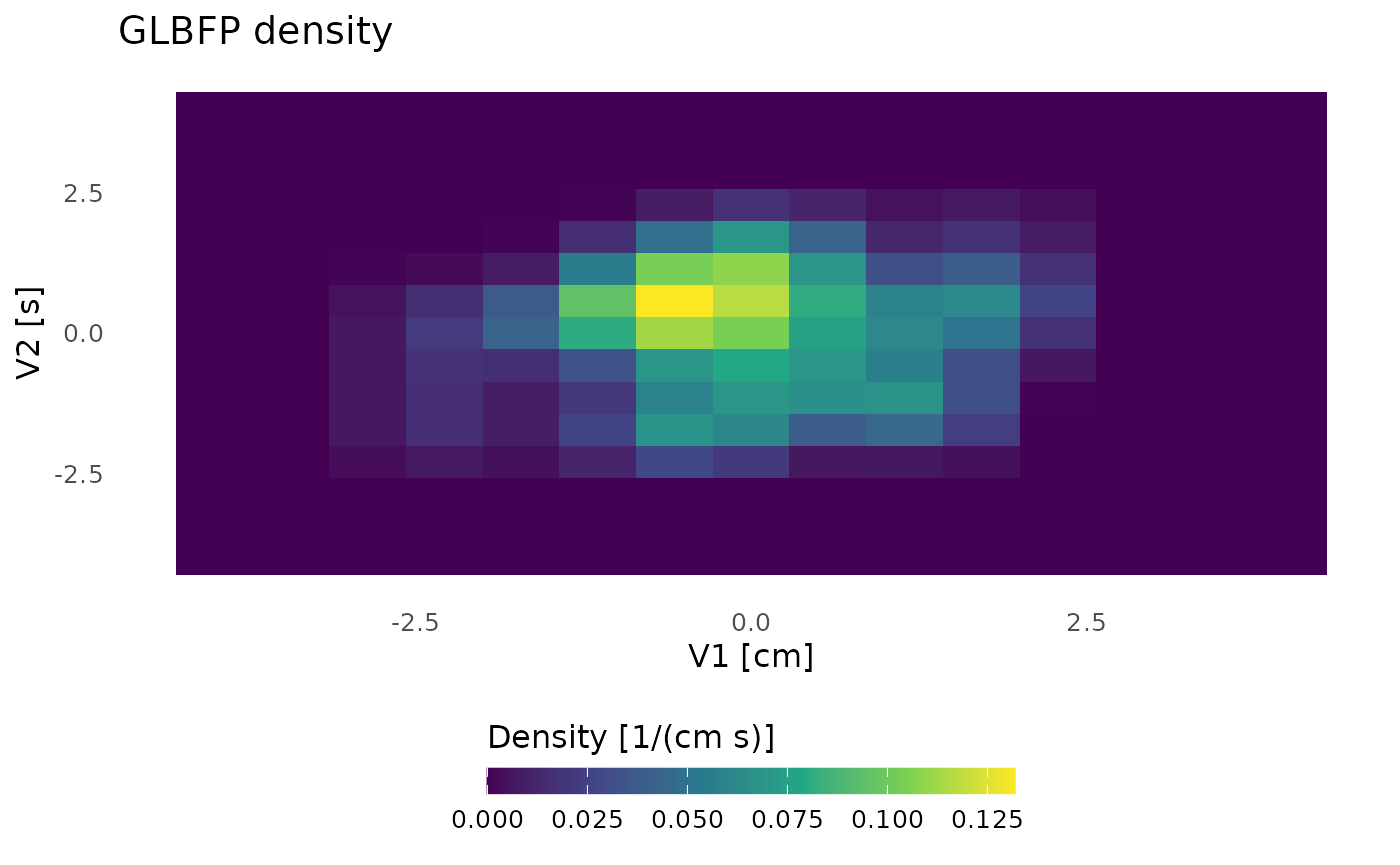

The heatmap above concerns $d=2$ observations on an $N=3$ field. A 3D surface of this fit uses density as its height. For $d=3$ , use joint-density slices or isosurfaces. Slices are not renormalized conditional densities.

For examples using real data, see the Quebec climate fields vignette. It illustrates $N=2$ and $N=3$ fields with $d=2$ observations.

References

Carbon, M. (2024). Le fameux GLBFP. Internal working note, Université Laval, été-automne 2024, equations (2)-(7), (22)-(36).

Carbon, M. and Duchesne, T. (2024). Multivariate frequency polygon for stationary random fields. Annals of the Institute of Statistical Mathematics 76, 263-287. https://doi.org/10.1007/s10463-023-00883-5.

Carbon, M. and Duchesne, T. (2026; online 2025). Asymptotic normality of multivariate frequency polygons for stationary random fields. Annals of the Institute of Statistical Mathematics 78, 297-326. https://doi.org/10.1007/s10463-025-00952-x.