Real Quebec climate fields: N=2 and N=3 • GLBFP

Data and two different dimensions

The bundled subset is extracted from ECCC’s CANGRD v2023 native grids. The data originate from homogenized station observations interpolated by ECCC. Each native cell is nominally 50 km wide. No further spatial interpolation, resampling, or imputation is performed in this example.

The two observation variables are anomalies of annual mean daily minimum and maximum temperatures, in degrees Celsius, relative to 1961-1990. Thus $d=2$ . The values are anomalies, not absolute temperatures or annual extreme values.

library(GLBFP)
library(ggplot2)
climate <- read.csv(system.file("extdata", "cangrd_quebec_1991_2020.csv", package = "GLBFP"))
head(climate[c("i", "j", "year", "tmin_anomaly_c", "tmax_anomaly_c")])
#>    i  j year tmin_anomaly_c tmax_anomaly_c
#> 1 91 26 1991           0.67           1.21
#> 2 90 27 1991           0.66           1.25
#> 3 91 27 1991           0.68           1.23
#> 4 92 27 1991           0.56           1.16
#> 5 90 28 1991           0.66           1.27
#> 6 91 28 1991           0.56           1.21

For 2020, sites are indexed by $(i,j)$ , so $N=2$ . For the 1991-2020 sequence, sites are indexed by $(i,j,\text{year})$ , so $N=3$ . Adding time changes the index dimension; it does not add a third observation variable.

values <- c("tmin_anomaly_c", "tmax_anomaly_c")
year2020 <- climate[climate$year == 2020L, ]
field2 <- glbfp_field(as.matrix(year2020[values]), as.matrix(year2020[c("i", "j")]),
  units = c("deg C", "deg C"), dependence = "dependent")
field3 <- glbfp_field(as.matrix(climate[values]), as.matrix(climate[c("i", "j", "year")]),
  units = c("deg C", "deg C"), dependence = "dependent")
field2
#> Indexed field: 92 observed sites; N = 2 ; d = 2 
#> Complete integer bounding box: FALSE 
#> Omitted sites: 0 ; dependence: dependent
field3
#> Indexed field: 2760 observed sites; N = 3 ; d = 2 
#> Complete integer bounding box: FALSE 
#> Omitted sites: 0 ; dependence: dependent

There are 92 sites and 2,760 site-years. The geographic selection is an incomplete subset of the native integer bounding box; it is not the outline of Quebec. All selected sites have both measurements for every selected year. No missing observations are filled. Latitude and longitude are retained as metadata and are not appended to the density variables.

Maps retain the native spatial resolution

map <- climate[climate$year %in% c(1991, 2005, 2020), ]
map$x_km <- (map$i - min(climate$i)) * 50
map$y_km <- (map$j - min(climate$j)) * 50
ggplot(map, aes(x_km, y_km, fill = tmin_anomaly_c)) +
  geom_tile(width = 50, height = 50) + coord_equal() + facet_wrap(~year) +
  scale_fill_viridis_c(name = "Tmin anomaly (deg C)") + theme_minimal() +
  labs(x = "Along native i-axis (km)", y = "Along native j-axis (km)",
       title = "Three time slices of the N=3 field") +
  theme(legend.position = "bottom")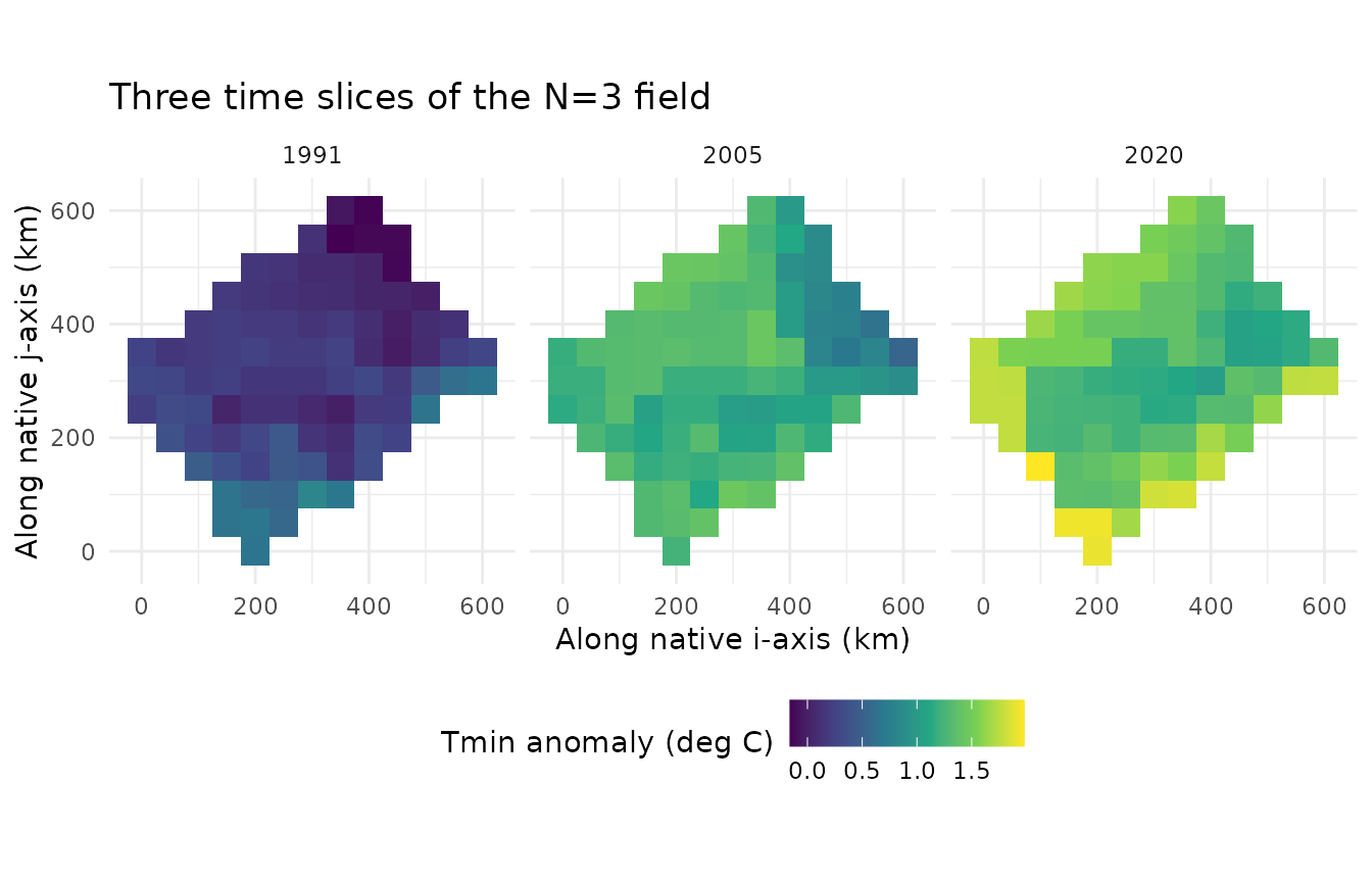

Each square represents an observed source-grid value, already interpolated by ECCC from stations. Smoothing its display would not add observed spatial detail. These are input maps, not GLBFP density estimates.

A bivariate density for either index dimension

Use common illustrative bandwidths $b=(0.6,0.6)$ , integers $m=(3,3)$ , fine counting-cell widths $b/m=(0.2,0.2)$ , and anchor $(-8,-8)$ , in temperature units. Counting cells are half-open, interpolation uses their centres, and unoccupied cells have zero counts on an unbounded lattice. Display limits do not clamp or renormalize the density.

points <- as.matrix(expand.grid(Tmin = seq(-3, 5, length.out = 201),
                               Tmax = seq(-3, 5, length.out = 201)))
fit2 <- GLBFP_estimate(field2, b = c(.6, .6), m = c(3, 3),
  min_vals = c(-8, -8), max_vals = c(8, 8), grid_points = points)
fit3 <- GLBFP_estimate(field3, b = c(.6, .6), m = c(3, 3),
  min_vals = c(-8, -8), max_vals = c(8, 8), grid_points = points)
plot_density(fit2, "heatmap", labels = c("Tmin anomaly", "Tmax anomaly"),
  title = "Bivariate density of the 2020 sites (N=2)") + coord_equal()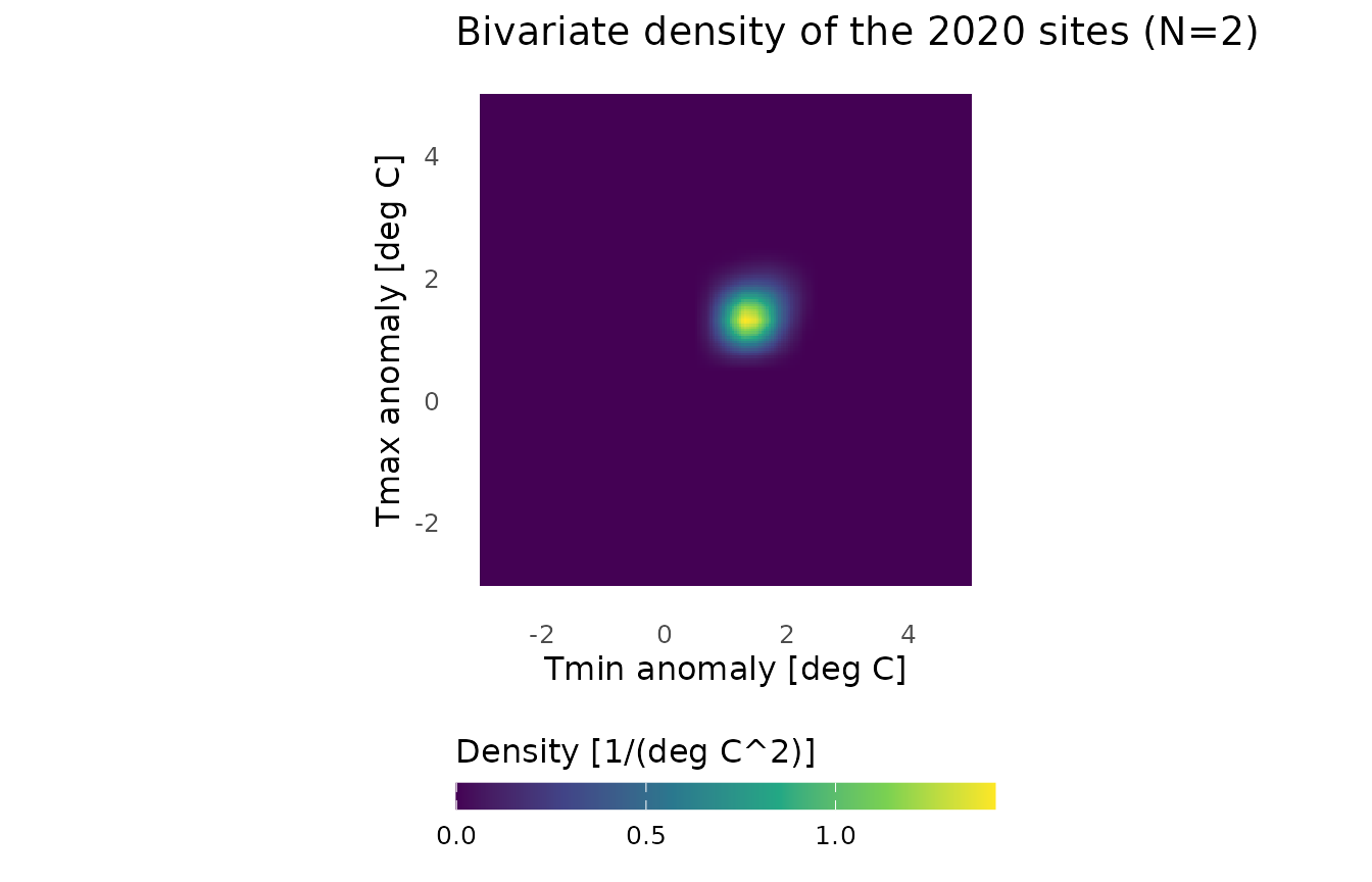

plot_density(fit3, "heatmap", labels = c("Tmin anomaly", "Tmax anomaly"),
  title = "Bivariate density of all selected site-years (N=3)") + coord_equal()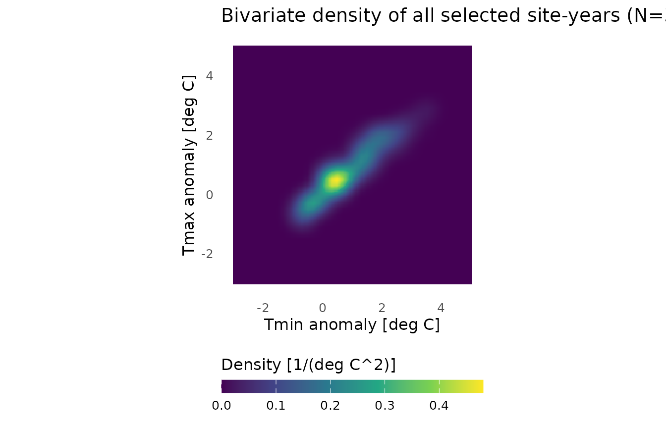

The density axes represent the two temperature anomalies. They do not represent geographic coordinates or time. A high density indicates a concentration of observed anomaly pairs. Density units are reciprocal squared degrees Celsius. A 3D surface would add density as its height while keeping $d=2$ . For true $d=3$ observations, use density slices or isosurfaces instead.

Pooling years gives equal weights to the selected site-years. This describes their finite mixture and does not assert a unique stationary climate law. There is no correction for geographic cell area; this example computes no confidence interval under dependence or calibrated climate-trend test. The bandwidth is illustrative, not claimed to be optimal. Dependence and interpolation uncertainty are not estimated by this demonstration.

Exports and provenance

The installed script exports refined density displays with 481 points per axis, contours, maps and self-contained interactive surfaces:

source(system.file("examples", "quebec_climate.R", package = "GLBFP"))

The denser evaluation grid changes the rendering, not the statistical counting grid. To estimate uncertainty, a justified dependence method would have to be specified separately; assigning integer spatial indices is not sufficient.

Data Source: Environment and Climate Change Canada. Contains information licenced under the Data Server End-use Licence of Environment and Climate Change Canada. No endorsement by ECCC is implied.

CANGRD documentation.
Data licence.
system.file("extdata", "cangrd_quebec_PROVENANCE.txt", package="GLBFP") gives extraction details and source hashes. The coordinates and years remain those of the native archive ctvb_cangrd_temp_v2023_Gen3.tar.gz.